Code
library(ivdtools)
library(readr)The diagnostic ability of a single marker is often limited; combining multiple markers can improve the overall discrimination. Besides single-marker ROC, the roc() function in ivdtools also supports combining multiple markers into a joint score with multivariate logistic regression (mlr()), computing its AUC, and predicting the positive probability for new samples.
This document demonstrates the joint analysis of two markers (x1, x2): first compare the single-marker AUCs, then fit a multivariate logistic regression model, draw the multi-curve ROC, and predict new samples. The AUC of the joint model on the training data is the apparent performance and should be validated on independent data before generalization; the reference variable must be binary.
library(ivdtools)
library(readr)| Function | Main purpose | Key input or output |
|---|---|---|
roc() |
Create a ROC object | cols supports multiple markers |
auc() |
Single-marker AUC | per column |
mlr() |
Multivariate logistic regression | cols, name; requires auc() first |
plot() |
ROC curve | mlr="all" overlays the joint-model curve |
predict() |
Predict positive probability | newdata, column_map |
summary() |
Summary |
mlr_dat <- read_csv("./data/roc-multimarker.csv", show_col_types = FALSE)
mlr_dat <- as.data.frame(mlr_dat)
str(mlr_dat)
'data.frame': 120 obs. of 4 variables:
$ sid: num 1 2 3 4 5 6 7 8 9 10 ...
$ ref: num 0 0 0 0 0 0 0 0 0 0 ...
$ x1 : num 5.51 3.19 8.13 6.16 11.12 ...
$ x2 : num 8.3 12.9 12.4 16.1 11.9 ...table(mlr_dat$ref)
 0  1
60 60
The data contain 120 cases (60 positive and 60 negative) and two quantitative markers, x1 and x2.
ro2 <- roc(mlr_dat, cols = c("x1", "x2"), reference = "ref", id = "sid")
ro2 <- auc(ro2)
AUC Table
  Column               AUC          95% CI  Direction
  ------------------------------------------------------------
  x1                0.9219  [0.8712, 0.9727]       geq
x2 0.8322 [0.7587, 0.9057] geqro2$auc_tableThe AUC of x1 is ≈ 0.922 and that of x2 is ≈ 0.832; among the single markers, x1 discriminates better.
Model jointly with both markers:
ro2 <- mlr(ro2, cols = c("x1", "x2"), name = "combined")
Multivariate Logistic Regression (combined)
  --------------------------------------------------
  Formula: reference_binary ~ x1 + x2
  n = 120  (positive = 60, negative = 60)
  AUC = 0.9642  [0.9298, 0.9985]

  Coefficients:
                   Estimate Std. Error   z value     Pr(>|z|)
    (Intercept) -13.6586717  2.7569949 -4.954188 7.263286e-07
    x1            0.7638502  0.1549103  4.930919 8.184356e-07
    x2            0.3949617  0.1064673  3.709700 2.075049e-04

  * Note: AUC is evaluated on the same data used for fitting;
the estimate may be optimistic.ro2$mlr_results$combined$fit_summary
Call:
glm(formula = formula, family = binomial, data = model_data)

Coefficients:
            Estimate Std. Error z value Pr(>|z|)
(Intercept) -13.6587     2.7570  -4.954 7.26e-07 ***
x1            0.7639     0.1549   4.931 8.18e-07 ***
x2            0.3950     0.1065   3.710 0.000208 ***
---
Signif. codes:  0 '***' 0.001 '**' 0.01 '*' 0.05 '.' 0.1 ' ' 1

(Dispersion parameter for binomial family taken to be 1)

    Null deviance: 166.355  on 119  degrees of freedom
Residual deviance:  58.112  on 117  degrees of freedom
AIC: 64.112

Number of Fisher Scoring iterations: 7ro2$mlr_results$combined$auc[1] 0.9641667The joint model has an AUC of ≈ 0.964 (95% CI [0.930, 0.999]), higher than either single marker, indicating that combining the two markers does provide a gain.
Parameter notes:
mlr(cols, name, ...)fits a binary logistic regression (glm) with the selected markers;nameis the model name (auto-generatesMLR01,MLR02, …);...is passed through toglm.auc()must be run first before callingmlr(). The coefficients are interpreted as log odds ratios; the joint AUC is computed on the data used for fitting and is an apparent performance.
plot(ro2, mlr = "all")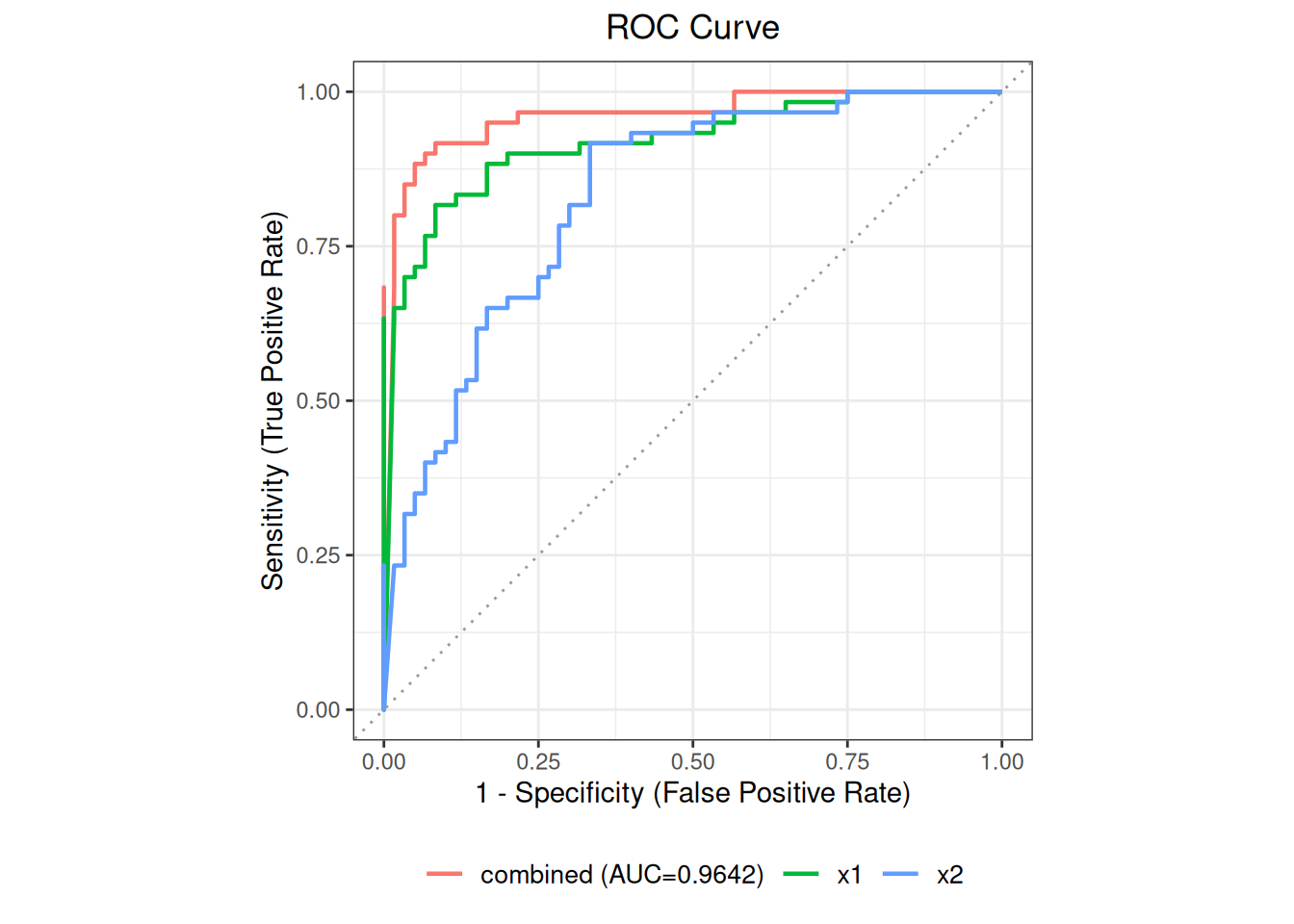
plot(ro2, mlr="all") draws the ROC curves of each single marker and the joint model together for comparison.
predict(ro2, newdata = data.frame(x1 = c(7, 12), x2 = c(16, 21)))predict() returns each predictor variable, the positive probability (pred_prob), the standard error and confidence interval, and the predicted class (pred_class) at the default threshold of 0.5. The two cases obtain positive probabilities of 0.12 and 0.98, respectively, consistent with the expected direction.
Parameter notes: When the column names of
newdatadiffer from those used in modeling, map them with the named vectorcolumn_map(for examplecolumn_map = c(new_x1 = "x1")). If the object contains multiple models,predict()must specify the model name withmlr.
summary(ro2)
ROC Analysis -- Summary
--------------------------------------------------

ROC Analysis
  Data class:        data.frame
  Total rows:        120
  Complete cases:    120
  Reference:         ref (binary)
  Positive / Neg:    60 / 60
  Evaluation cols:   2  (x1, x2)
  Duplicate IDs:     none

Analysis slots:
    [ ] Describe
    [x] AUC
    [ ] Cutoff
    [x] MLR


AUC Table
  Column               AUC          95% CI  Direction
  ------------------------------------------------------------
  x1                0.9219  [0.8712, 0.9727]       geq
  x2                0.8322  [0.7587, 0.9057]       geq

MLR Results

Multivariate Logistic Regression (combined)
  --------------------------------------------------
  Formula: reference_binary ~ x1 + x2
  n = 120  (positive = 60, negative = 60)
  AUC = 0.9642  [0.9298, 0.9985]

  Coefficients:
                   Estimate Std. Error   z value     Pr(>|z|)
    (Intercept) -13.6586717  2.7569949 -4.954188 7.263286e-07
    x1            0.7638502  0.1549103  4.930919 8.184356e-07
    x2            0.3949617  0.1064673  3.709700 2.075049e-04

  * Note: AUC is evaluated on the same data used for fitting;
the estimate may be optimistic.mlr() fits a given set of markers in one call; comparisons of multiple variable sets should be pre-specified in the protocol to avoid repeated trial and error.