4 Stability Studies

4.1 Analysis Objectives

Stability studies evaluate the extent to which measurement results change over time for reagents, calibrators, or quality-control materials under specified storage, transport, or use conditions. This document demonstrates how to use the ivdtools package to establish a stability analysis plan, complete node bias, regression of trends within and between conditions relative to the first node, prediction of the time to reach an allowable limit, Arrhenius accelerated stability analysis, and mean kinetic temperature (MKT) computation.

Code

library(ivdtools)
library(readr)

All data in this document are deterministic teaching examples used only to validate the analysis workflow. The 5% allowable drift, 10% accelerated degradation limit, target temperature, and activation energy in the examples are not universal acceptance criteria; formal studies must use parameters pre-specified in the protocol, risk assessment, or applicable standards. Whether to choose a concentration value or a signal value as the response should be decided according to the protocol.

4.2 Overview of Functions

Function	Main purpose	Key input or output
`stability_plan()`	Plan the minimum number of time points for a regression series	Allowable drift, variability, replicates, expected drift and power
`stability_bias()`	Compute absolute/relative bias of each condition relative to the first node	Node summary, within-condition bias, between-condition bias and limit status
`stability_regression()`	Regression of a single-condition trend or test/reference paired bias	Slope, one-sided confidence limit, node results and diagnostics
`stability_time()`	Predict the time when the point estimate or one-sided confidence limit reaches the allowable bias	Predicted time, whether extrapolated, and search range
`arrhenius()`	Extrapolate the shelf life at target temperature from degradation rates at multiple elevated temperatures	Kinetic order, rate, activation energy and predicted shelf life
`mkt()`	Compute equally spaced or time-weighted mean kinetic temperature	Per-probe and combined MKT

stability_regression() supports two modes:

mode = "self": regress the measurement results of a single condition over time;
mode = "compare": compute the bias of the test condition relative to the reference condition at matched time points, then regress the bias over time.

Before analysis, clarify the condition mapping, time unit, bias scale, expected direction of change, and allowable limits. Conclusions about acceptability can be drawn only when the protocol provides acceptance criteria.

4.3 Example 1: Establishing an Analysis Plan

Suppose the study protocol specifies an allowable relative drift of 5%, an expected drift of 2.5%, repeatability variability of 1.5%, and a target power of 90%. Compare the minimum number of time points needed when measuring 1, 2, or 3 times at each time point:

Code

plan <- ivdtools::stability_plan(
  allowable_drift = 5,
  variability = 1.5,
  replicates = c(1, 2, 3),
  expected_drift = 2.5,
  power = 0.9,
  mode = "simple",
  bias_type = "relative"
)
print(plan)


Stability Study Time-Point Plan
  Allowable drift: 5.0000; expected drift: 2.5000
  Success target:  90%; method: CLSI EP25 Appendix A Table A2

  Replicates     Residual  Allow/Resid  Min nodes
  ------------------------------------------------
           1       1.5000       3.3333        n/a
           2       1.0607       4.5455         28
           3       0.8660       5.7471         18

  n/a -- No feasible entry in EP25 table.

4.4 Example 2: Bias Analysis

4.4.1 Reading and Validating Raw Data

Code

bias_data <- read_csv(
  "./data/stability-bias-example.csv",
  show_col_types = FALSE
)
bias_data

Code

dim(bias_data)

[1] 30  4

Code

str(bias_data)

spc_tbl_ [30 × 4] (S3: spec_tbl_df/tbl_df/tbl/data.frame)
 $ Condition: chr [1:30] "2-8C" "2-8C" "2-8C" "2-8C" ...
 $ Day      : num [1:30] 0 0 0 7 7 7 14 14 14 21 ...
 $ Replicate: num [1:30] 1 2 3 1 2 3 1 2 3 1 ...
 $ Result   : num [1:30] 100.2 99.8 100 99.9 100.1 ...
 - attr(*, "spec")=
  .. cols(
  ..   Condition = col_character(),
  ..   Day = col_double(),
  ..   Replicate = col_double(),
  ..   Result = col_double()
  .. )
 - attr(*, "problems")=<externalptr>

4.4.2 Node Bias Computation

Using 2-8C as the reference condition, normalize to each condition’s own first node, and evaluate whether the relative bias is within the illustrative ±5% limit:

Code

bias_result <- ivdtools::stability_bias(
  data = bias_data,
  condition = "Condition",
  time = "Day",
  value = "Result",
  reference_condition = "2-8C",
  limit = 5,
  bias_type = "relative",
  time_unit = "d"
)
print(bias_result)


Stability Bias Analysis
  Conditions:      2 (2-8C, 25C)
  Reference:       2-8C
  Time unit:       d
  Node comparisons:20
  Acceptance:      +/- 5.0000 (relative); 10/10 nodes passed

  Within-condition bias (vs first node)
  Cond         Time      Value    Bias(%) Status
  ----------------------------------------------
  2-8C       0.0000   100.0000     0.0000 Pass
  2-8C       7.0000    99.9333    -0.0667 Pass
  2-8C      14.0000    99.7333    -0.2667 Pass
  2-8C      21.0000    99.5000    -0.5000 Pass
  2-8C      28.0000    99.3333    -0.6667 Pass
  25C        0.0000   100.0000     0.0000 Pass
  25C        7.0000    99.2333    -0.7667 Pass
  25C       14.0000    98.3333    -1.6667 Pass
  25C       21.0000    97.2333    -2.7667 Pass
  25C       28.0000    95.8333    -4.1667 Pass

  Between-condition bias (reference: 2-8C)
      Time Condition    TestVal  Bias(%)
  --------------------------------------
    0.0000 25C        100.0000     0.0000
    7.0000 25C         99.2333    -0.7005
   14.0000 25C         98.3333    -1.4037
   21.0000 25C         97.2333    -2.2781
   28.0000 25C         95.8333    -3.5235

Within-condition bias uses each condition’s own first node as the baseline; between-condition bias compares the test and reference conditions at the same time points.

Code

plot(bias_result)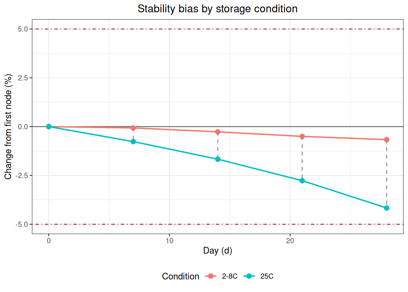

4.5 Example 3: Regression Analysis Comparing Storage Conditions

4.5.1 Reading and Validating Raw Data

Code

regression_data <- read_csv(
  "./data/stability-regression-example.csv",
  show_col_types = FALSE
)
regression_data

4.5.2 Comparing Test and Reference Conditions

Compute the relative bias of 25C relative to 2-8C at each matched time point, and regress the bias over time. The example pre-specifies that results decrease over time, so direction = "decrease" is used:

Code

regression_result <- ivdtools::stability_regression(
  data = regression_data,
  time = "Day",
  value = "Result",
  condition = "Condition",
  mode = "compare",
  test_condition = "25C",
  reference_condition = "2-8C",
  bias_type = "relative",
  direction = "decrease",
  conf.level = 0.95,
  limit = 5,
  time_unit = "d"
)
print(regression_result)


Stability Regression
  Mode:            compare
  Test condition:  25C
  Reference:       2-8C
  Fit:             WLS (1/SE^2); intercept = 0.0799, slope = -0.1025
  Direction:       decrease
  One-sided CI:    95.0%
  R-squared:       0.9956
  Cook distance:   row(s) 6 > 1; not removed

      Time      ObsBias   Estimate   CI_limit Status
  --------------------------------------------------
    0.0000       0.0000     0.0799    -0.0750       
    7.0000      -0.6669    -0.6376    -0.7566       
   14.0000      -1.3013    -1.3552    -1.4522       
   21.0000      -2.0040    -2.0728    -2.1717       
   28.0000      -2.6747    -2.7904    -2.9140       
   42.0000      -4.3842    -4.2256    -4.4296

Code

plot(regression_result)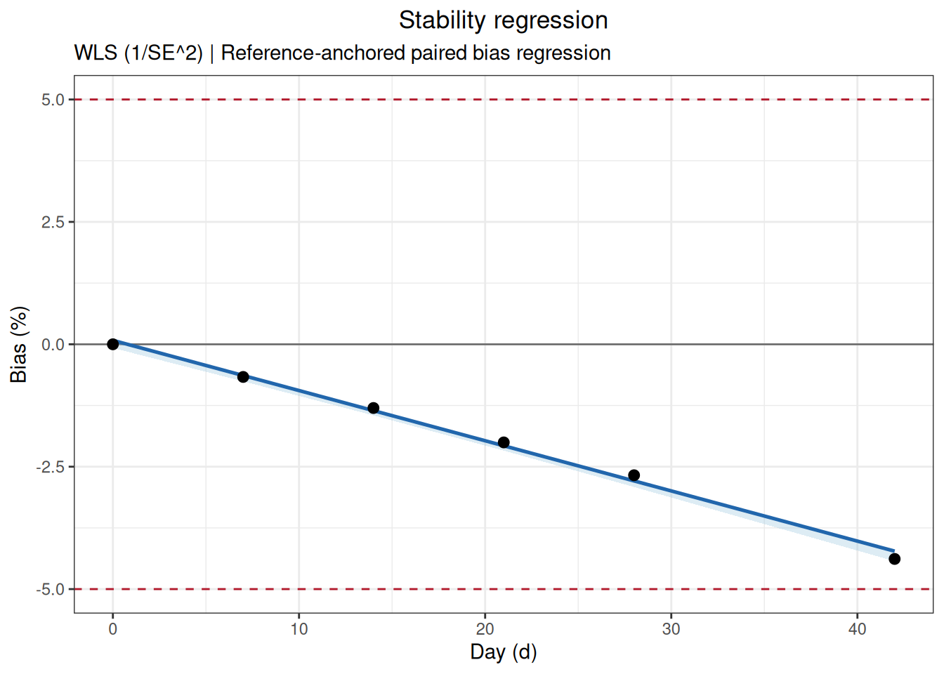

The model uses a one-sided confidence limit to evaluate the least favorable direction. This example identifies a node with a large Cook’s distance, but the function does not automatically delete it; you should go back to the original records, experimental procedure, and protocol requirements, and perform an include/exclude sensitivity analysis when there is sufficient justification.

4.6 Example 4: Regression Analysis Relative to the First Node

4.6.1 Single-Condition Analysis Relative to the First Node

In addition to the test/reference paired regression of Example 3, mode = "self" can analyze how a single condition changes over time on its own. The regression example data is still used below, but only the 25C condition is selected; the observed_bias at each node is computed relative to that condition’s first-node mean:

Code

self_regression_result <- ivdtools::stability_regression(
  data = regression_data,
  time = "Day",
  value = "Result",
  condition = "Condition",
  mode = "self",
  test_condition = "25C",
  bias_type = "relative",
  direction = "decrease",
  conf.level = 0.95,
  limit = 5,
  time_unit = "d"
)
print(self_regression_result)


Stability Regression
  Mode:            self
  Test condition:  25C
  Fit:             WLS (1/SE^2); intercept = 100.0849, slope = -0.1115
  Direction:       decrease
  One-sided CI:    95.0%
  R-squared:       0.9966
  Cook distance:   row(s) 1, 6 > 1; not removed

      Time      ObsBias   Estimate   CI_limit Status
  --------------------------------------------------
    0.0000       0.0000    -0.0000    -0.0000       
    7.0000      -0.7000    -0.7797    -0.8278       
   14.0000      -1.4000    -1.5594    -1.6555       
   21.0000      -2.2000    -2.3391    -2.4833       
   28.0000      -2.9667    -3.1188    -3.3110       
   42.0000      -4.7667    -4.6782    -4.9665

Code

plot(self_regression_result)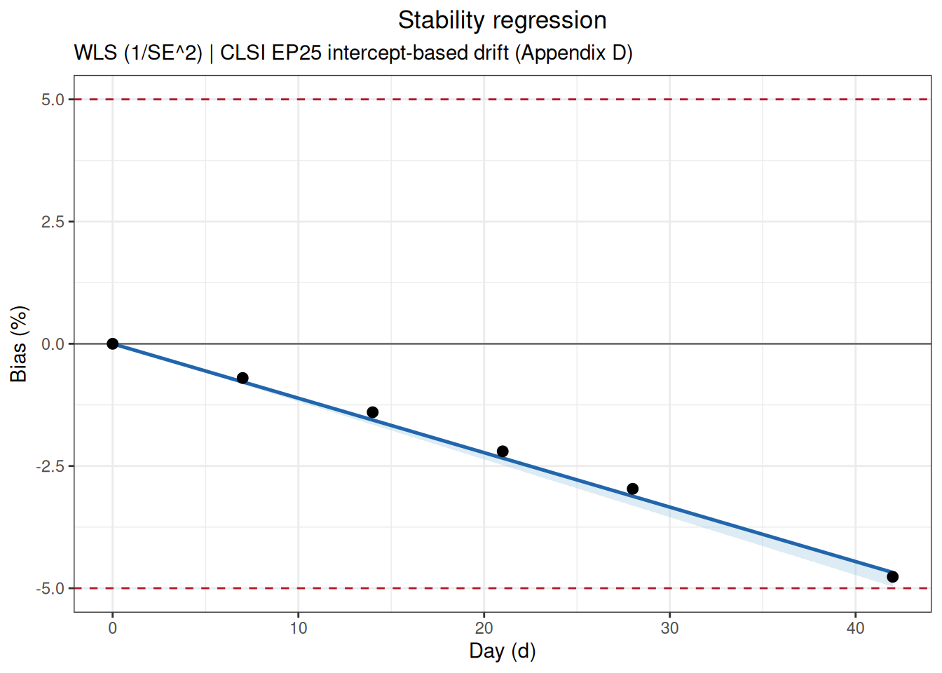

The observed bias at the first node is fixed at 0; the model estimates, however, are fitted jointly from all time points and do not require the regression intercept to pass exactly through the first node. A one-sided confidence limit is used to evaluate the pre-specified least favorable direction; the illustrative ±5% limit still cannot replace the study protocol requirements.

4.7 Example 5: Predicting the Time to Reach a Limit

stability_time() uses the regression object from Example 3 to compute the times at which the point estimate and the one-sided confidence limit first reach a -5% bias:

Code

time_result <- ivdtools::stability_time(
  regression_result,
  limit = 5,
  max_time = 90
)
print(time_result)


Stability Limit Time
  Limit: 5.0000 (relative); direction: decrease
  estimate       49.5548 d [EXTRAPOLATED]
  one_sided_ci   47.2316 d [EXTRAPOLATED]

Code

plot(time_result)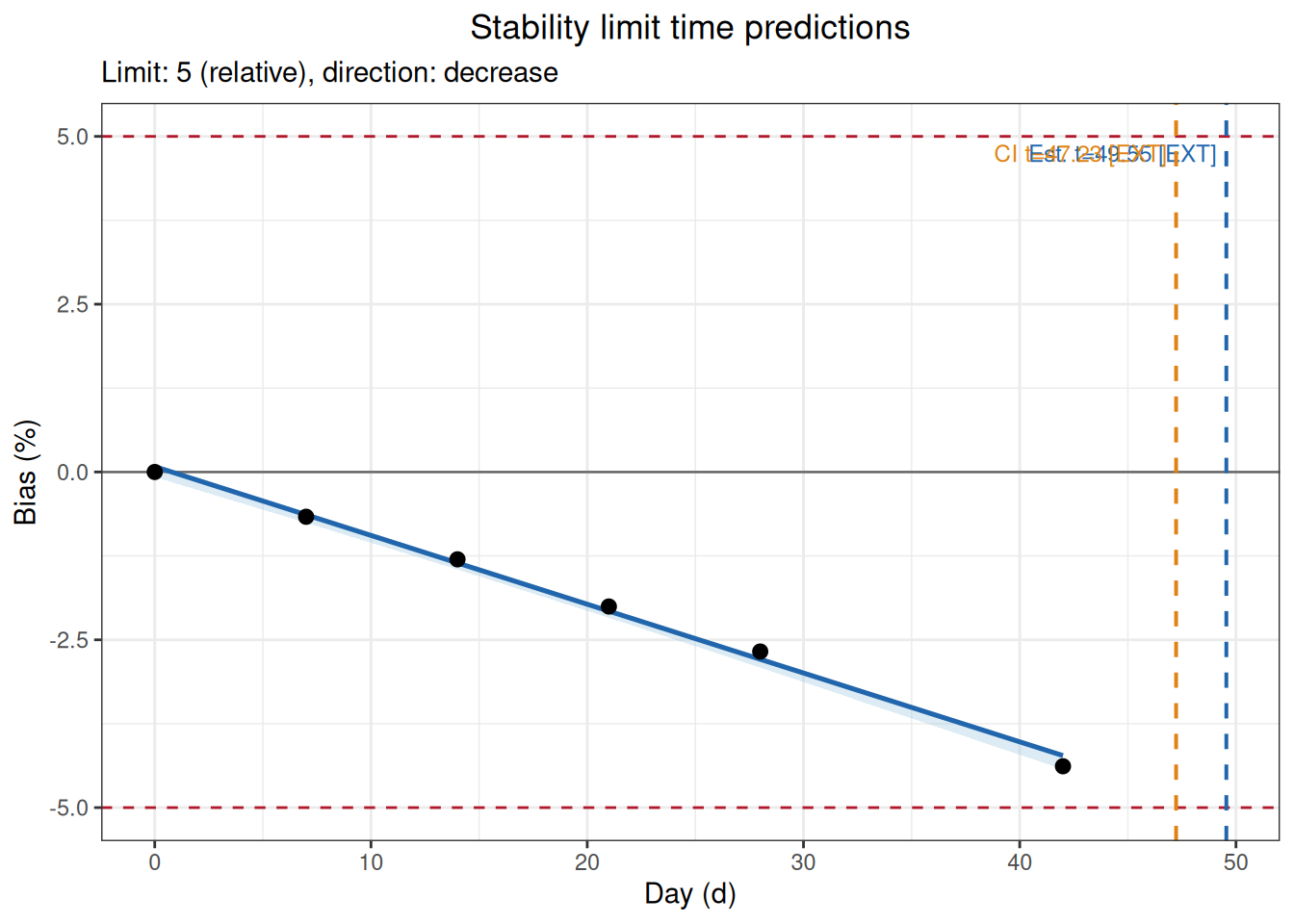

In this example, the longest actual observation time is 42 days, while the predicted time to reach the limit exceeds the observation range, so the output is marked EXTRAPOLATED. Extrapolated results rely on the assumption that the linear trend continues beyond the unobserved interval and cannot be treated as measured stability evidence; report the extrapolation distance and uncertainty prominently, and prefer confirmation with longer actual observation data.

4.8 Example 6: Arrhenius Accelerated Stability Analysis

4.8.1 Reading and Validating Raw Data

Code

arrhenius_data <- read_csv(
  "./data/stability-arrhenius-example.csv",
  show_col_types = FALSE
)
arrhenius_data

4.8.2 Kinetic and Arrhenius Fitting

The example uses accelerated data at 30, 37, and 45 °C, extrapolated to 5 °C; allows a relative change of 10%, and pre-specifies the degradation direction as decreasing:

Code

arrhenius_result <- ivdtools::arrhenius(
  data = arrhenius_data,
  temperature = "Temperature",
  time = "Day",
  value = "Result",
  target_temp = 5,
  order = "auto",
  direction = "decrease",
  limit = 10,
  bias_type = "relative",
  temp_unit = "C",
  time_unit = "d",
  conf.level = 0.95
)
print(arrhenius_result)


Arrhenius Stability Analysis
  Kinetic order:   zero (auto-selected)
  Direction:       decrease
  Activation Ea:   97.159 kJ/mol
  Target rate:     0.002346 /d
  Limit time:      4263.7878 d [1585.3589, 11467.3633]

Code

plot(arrhenius_result)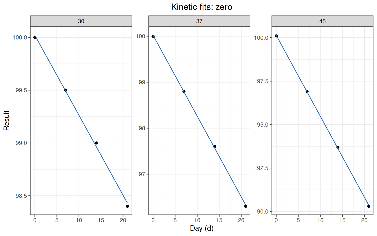

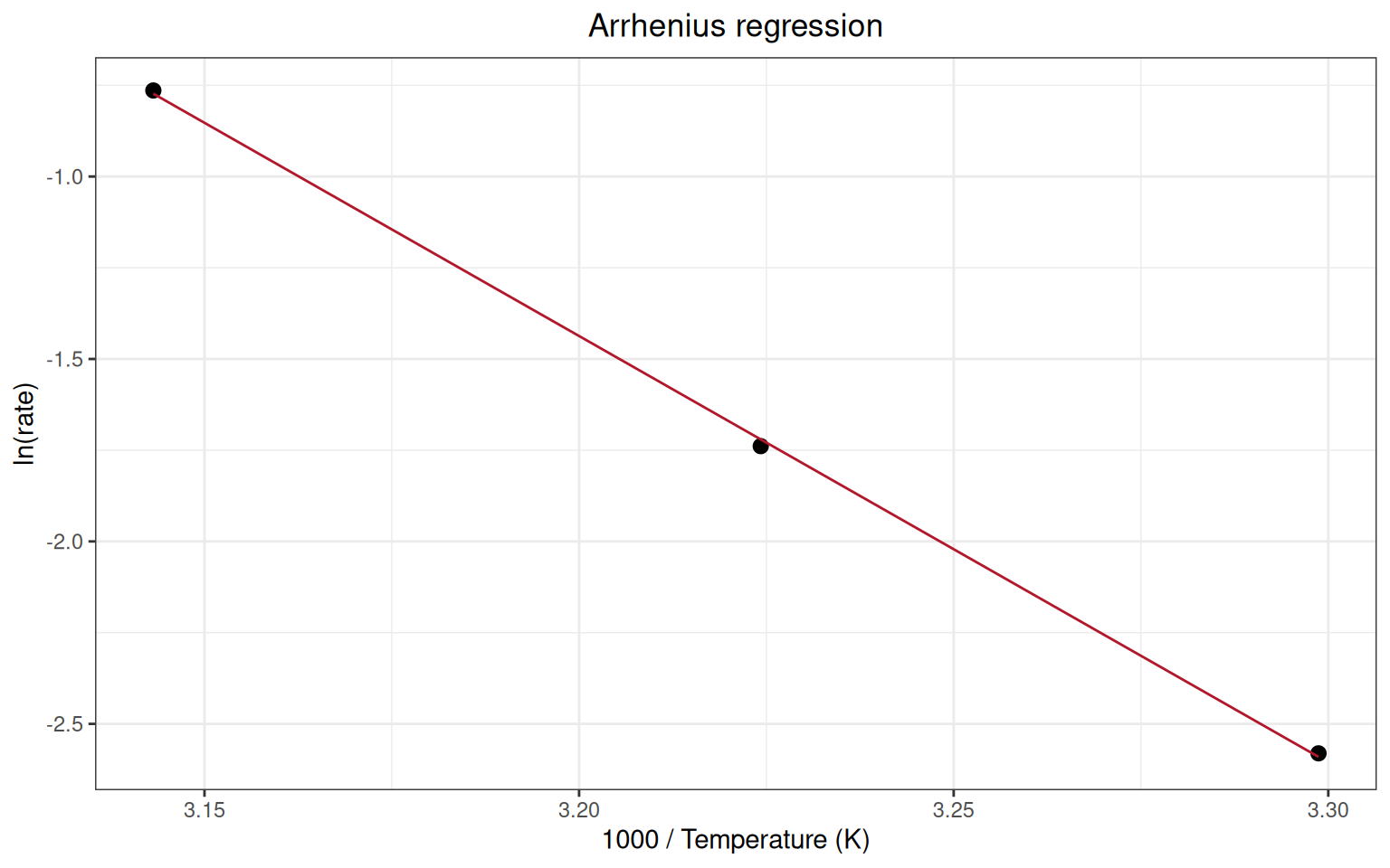
order = "auto" selects a model from the zero-order and first-order kinetic candidates according to the implementation rules. Formal analysis should determine the candidate orders under experimental design and mechanistic knowledge, and verify the degradation direction, rate significance, extent of degradation, and model residuals at each temperature. Extrapolating from elevated temperatures to the target storage temperature may span a large range; the predicted shelf life and its interval must be interpreted together with the model assumptions, the actual time data, and validation studies.

4.9 Example 7: MKT Computation

4.9.1 Reading and Validating Raw Temperature Data

Code

mkt_data <- read_csv(
  "./data/stability-mkt-example.csv",
  show_col_types = FALSE
)
mkt_data$Timestamp <- as.POSIXct(
  mkt_data$Timestamp,
  format = "%Y-%m-%d %H:%M:%S",
  tz = "UTC"
)
mkt_data

4.9.2 Time-Weighted MKT

Using two temperature probes and the actual time intervals, with temperature in degrees Celsius and an example activation energy of 83.144 kJ/mol:

Code

mkt_result <- ivdtools::mkt(
  data = mkt_data,
  temp_cols = c("Probe_A", "Probe_B"),
  time = "Timestamp",
  temp_unit = "C",
  ea = 83.144
)
print(mkt_result)


Mean Kinetic Temperature
  Ea: 83.144 kJ/mol
  Method: Time-weighted trapezoidal MKT

  Probe_A              299.538 K     26.388 C
  Probe_B              299.194 K     26.044 C
  Combined             299.367 K     26.217 C

MKT is not a simple arithmetic mean of temperature; high-temperature exposure receives greater weight through the Arrhenius relationship. Formal computations should confirm probe calibration status, time ordering, missing intervals, temperature units, exposure duration, and the activation energy assumption. MKT can only summarize temperature exposure; it cannot replace product-specific stability studies.

4.10 Splitting Multi-Sample Data

When different concentration levels, sample types, or lots need to be evaluated separately, you should retain the sample identifier, split the data first, and then analyze each sample with the same pre-specified parameters. Read and validate the multi-sample raw data:

Code

multiple_samples_data <- read_csv(
  "./data/stability-multiple-samples-example.csv",
  show_col_types = FALSE
)
multiple_samples_data

Use split() to build a list of data named by sample, and first look at one of the samples:

Code

sample_data_list <- split(
  multiple_samples_data,
  multiple_samples_data$Sample
)
names(sample_data_list)

[1] "Sample_A" "Sample_B"

Code

sample_a_data <- sample_data_list[["Sample_A"]]
sample_a_data

Perform the analysis on each sample in turn.

4.11 Key Points for Interpreting Results

Protocol first: Before analysis, specify conditions, nodes, replicates, time units, direction, bias scale, and acceptance limits.
Raw data read-only: Report missing, duplicate, non-numeric records, and every excluded row at each step; do not automatically delete anomalous records.
Correct pairing: Condition comparisons must be made at matched time points, with the test and reference conditions explicitly identified.
Model diagnostics: Report slope, confidence limits, fitting method, residuals, influential points, and whether a WLS fallback occurred.
Prominent extrapolation: Predictions of stability time beyond the observed range should be clearly labeled and not treated as measured evidence.
Explicit temperature assumptions: Arrhenius analysis and MKT must record Celsius/Kelvin units, time units, and activation energy.
Separate statistics from acceptability: Statistical significance is not the same as product acceptability; judgments can only be based on pre-specified allowable limits.
Independent review: Clinical, regulatory, or release decisions should be independently reviewed by appropriate professionals.