12  Method Comparison

12.1 Analysis Objectives

Method comparison evaluates the agreement between the results measured on the same samples by a candidate method and a reference method, corresponding to CLSI EP09. The mcr() function in ivdtools provides a progressive S3 workflow: descriptive statistics → correlation analysis → regression (OLS, WLS, Deming, weighted Deming, Passing–Bablok) → Bland–Altman → outliers → bias at medical decision levels, and provides plotting, prediction, and summarization. This document demonstrates the full workflow with a complete example containing different lots and sample types, and demonstrates subgroup comparison after splitting by lot/sample type.

The example data are deterministic teaching data, into which an outlier has been deliberately added to demonstrate outlier detection; statistical results do not automatically constitute a pass/fail determination; acceptance criteria should be defined before analysis.

library(ivdtools)
library(readr)

12.2 Overview of Functions

Function	Main purpose	Key input or output
mcr()	Create a method-comparison object	id, candidate, reference, weights
describe()	Descriptive statistics	candidate/reference/difference and extra columns
correlation()	Correlation analysis	pearson/spearman/kendall
regression()	Regression fitting	ols/wls/deming/wdeming/pb, lambda, weights
bland_altman()	Agreement limits	difference/ratio/percent, x_axis
outlier()	Difference outlier	grubbs/esd/dixon/iqr, type
bias()	Bias at medical decision levels	mdl, interval
predict()	Forward/inverse prediction	requires regression first
plot() / summary()	Graphics and summary	type selects the graphic

12.3 Example: A Complete Single-Sample Analysis

12.3.1 Reading and Validating Data

The data contain 40 cases, each with an ID id, candidate method result candidate, reference method result reference, as well as a lot batch (B1/B2) and a sample type sample_type (serum/plasma/urine):

mc_dat <- read_csv("./data/method-comparison.csv", show_col_types = FALSE)
mc_dat <- as.data.frame(mc_dat)
str(mc_dat)

'data.frame':   40 obs. of  5 variables:
 $ id         : num  1 2 3 4 5 6 7 8 9 10 ...
 $ batch      : chr  "B1" "B1" "B1" "B1" ...
 $ sample_type: chr  "serum" "plasma" "urine" "serum" ...
 $ reference  : num  10 14.9 19.7 24.6 29.5 34.4 39.2 44.1 49 53.8 ...
 $ candidate  : num  11.6 16.6 20.9 30.4 34 ...

dim(mc_dat)

[1] 40  5

knitr::kable(table(mc_dat$batch), caption = "Lot distribution")

Lot distribution

Var1	Freq
B1	20
B2	20

knitr::kable(table(mc_dat$sample_type), caption = "Sample type distribution")

Sample type distribution

Var1	Freq
plasma	13
serum	14
urine	13

12.3.2 Creating the Object and Descriptive Statistics

mc <- mcr(mc_dat, id = "id", candidate = "candidate", reference = "reference")

mc <- describe(mc, cols = c("batch", "sample_type"))

Descriptive Statistics
  Variable               n     Mean       SD      Min       Q1   Median       Q3      Max  NA
  --------------------------------------------------------------------------- 
    candidate (X)       40 112.4977  59.2513  11.5900  63.1075 112.5750 159.5925 209.9000  
    reference (Y)       40 105.0000  56.9555  10.0000  57.4750 105.0000 152.5250 200.0000  
    Diff (X-Y)          40   7.4977   3.9583   1.2000   5.2725   6.6100   9.7950  22.1000  

  batch
  Level                Count  Percent
   -------------------------------------- 
  B1                      20    50.0%
  B2                      20    50.0%

  sample_type
  Level                Count  Percent
   -------------------------------------- 
  plasma                  13    32.5%
  serum                   14    35.0%
  urine                   13    32.5%

mc

Method Comparison
  Data class:        data.frame
  Total rows:        40
  Complete pairs:    40
  ID variable:       id
  Test method (X):   candidate
  Reference (Y):     reference
  Duplicate IDs:     none

Analysis slots:
    [x] Describe
    [ ] Correlation
    [ ] Regression
    [ ] Outlier
    [ ] Bland-Altman
    [ ] Bias

The cols of describe() specifies the categorical/numeric extra columns to include in the description, and supports exclusion with a - prefix.

12.3.3 Correlation Analysis

mc <- correlation(mc, method = "pearson")

Correlation
  Method: pearson
  r = 0.9985, 95% CI [0.9971, 0.9992]
  p-value: < 2.2e-16
  n = 40

Parameter notes: The method of correlation() can be "pearson", "spearman", or "kendall". Correlation reflects the degree to which the two variables co-vary; it is not the same as agreement and cannot replace Bland–Altman or regression bias evaluation.

12.3.4 Regression Analysis

Compare OLS, Deming, Passing–Bablok, and WLS in turn. Because regression() updates the regression result within the object, the multiple methods are stored in separate objects for comparison:

mc_ols <- regression(mc, method = "ols")

Regression
  Method: OLS
  Intercept = -2.9723  (SE = 1.0971)
  Slope     = 0.9598  (SE = 0.0087)
  Intercept 95% CI: [-5.1933, -0.7513]
  Slope     95% CI: [0.9423, 0.9773]
    H0: slope = 1 -> t = -4.6494, p = 3.944e-05
    slope significantly different from 1 (CI excludes 1)
  R-squared = 0.9969
  Sigma     = 3.2015
  n = 40

mc_dem <- regression(mc, method = "deming")

Regression
  Method: Deming
  Intercept = -3.1323  (SE = 1.4133)
  Slope     = 0.9612  (SE = 0.0092)
  Intercept 95% CI: [-5.9934, -0.2712]
  Slope     95% CI: [0.9426, 0.9798]
    H0: slope = 1 -> t = -4.2313, p = 0.0001413
    slope significantly different from 1 (CI excludes 1)
  Sigma     = 3.2026
  n = 40

mc_pb  <- regression(mc, method = "pb")

Regression
  Method: Passing-Bablok
  Intercept = -2.1674  (SE =    NA)
  Slope     = 0.9556  (SE =    NA)
  Intercept 95% CI: [-3.1487, -0.9828]
  Slope     95% CI: [0.9444, 0.9669]
  Sigma     = 3.2299
  n = 40

mc_wls <- regression(mc, method = "wls", weights = "1/y")

Regression
  Method: WLS
  Weights: 1/y
  Intercept = -2.2924  (SE = 0.9153)
  Slope     = 0.9518  (SE = 0.0108)
  Intercept 95% CI: [-4.1452, -0.4396]
  Slope     95% CI: [0.9299, 0.9736]
    H0: slope = 1 -> t = -4.4712, p = 6.818e-05
    slope significantly different from 1 (CI excludes 1)
  R-squared = 0.9951
  Sigma     = 0.4819
  n = 40

knitr::kable(
  data.frame(
    Method = c("OLS", "Deming", "Passing-Bablok", "WLS(1/y)"),
    Intercept = c(mc_ols$regression$intercept, mc_dem$regression$intercept,
             mc_pb$regression$intercept, mc_wls$regression$intercept),
    Slope = c(mc_ols$regression$slope, mc_dem$regression$slope,
             mc_pb$regression$slope, mc_wls$regression$slope)
  ),
  digits = 4,
  caption = "Intercept and slope comparison across the four regression methods"
)

Intercept and slope comparison across the four regression methods

Method	Intercept	Slope
OLS	-2.9723	0.9598
Deming	-3.1323	0.9612
Passing-Bablok	-2.1674	0.9556
WLS(1/y)	-2.2924	0.9518

print(mc_ols)

Method Comparison
  Data class:        data.frame
  Total rows:        40
  Complete pairs:    40
  ID variable:       id
  Test method (X):   candidate
  Reference (Y):     reference
  Duplicate IDs:     none

Analysis slots:
    [x] Describe
    [x] Correlation (pearson)
    [x] Regression (OLS)
    [ ] Outlier
    [ ] Bland-Altman
    [ ] Bias

In this example, the OLS slope is ≈ 0.96, and its 95% CI does not contain 1, indicating that the candidate method has about a 4% proportional bias (the true bias in the data is 5%).

Parameter notes: The method of regression() can be "ols", "wls", "deming", "wdeming", or "pb". Deming uses lambda to specify the variance ratio (ref/cand, default 1); wls/wdeming must provide weights (a built-in scheme or a data column name); conf.level controls the parameter confidence interval.

12.3.5 Bias at Medical Decision Levels

Use bias() to evaluate the predicted bias at medical decision levels (MDL):

mc_ols <- bias(mc_ols, mdl = c(30, 80, 150), interval = "both")

Bias
  Method: OLS
  Interval: both (95%)
  MDL points: 3
  Bias range: [4.1791, 9.0064]

 mdl     bias ci_lower  ci_upper  pi_lower pi_upper 
--------------------------------------------------- 
  30 4.179112 2.407658  5.950566 -2.539698 10.89792
  80 6.190463 5.018240  7.362685 -0.395770 12.77670
 150 9.006354 7.789153 10.223554  2.411967 15.60074 

mc_ols$bias

plot(mc_ols, type = "bias", mdl = c(30, 80, 150))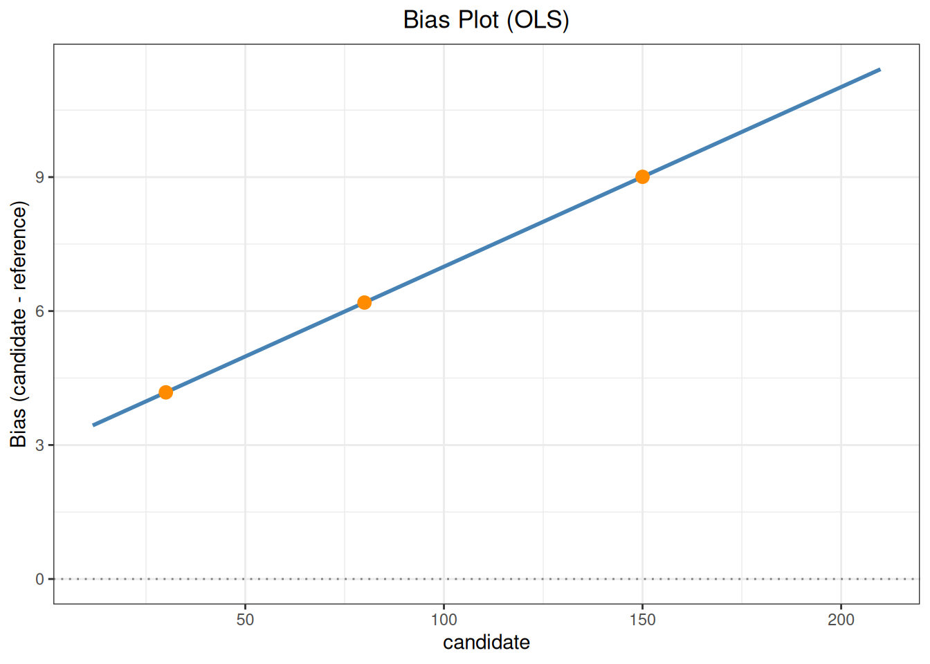

Parameter notes: In bias(mdl, level, interval), mdl is a vector of medical decision levels; interval can be "", "confidence", "prediction", or "both". Bias is defined as the difference between the fitted value of the candidate method at mdl and mdl; interpret it together with the regression direction and the allowable bias specified in the protocol.

12.3.6 Bland–Altman Analysis

mc_ols <- bland_altman(mc_ols, type = "difference")

Bland-Altman
  Type:        difference
  Y-axis:      candidate - reference
  X-axis:      Mean of candidate and reference
  n = 40

  Mean diff:       7.4977
  SD diff:         3.9583
  95% LoA: [-0.2603, 15.2558]

  95% CI for LoA:
    Lower LoA: [-2.4419, 1.9213]
    Upper LoA: [13.0742, 17.4374]

plot(mc_ols, type = "bland_altman")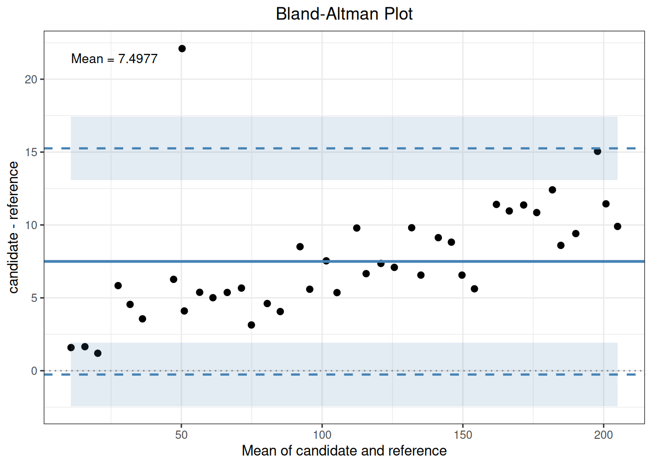

mc_ols$bland_altman[c("mean_diff", "sd_diff", "loa")]

$mean_diff
[1] 7.49775

$sd_diff
[1] 3.958259

$loa
     lower      upper 
-0.2602947 15.2557947 

Parameter notes: The type of bland_altman() can be "difference", "ratio", or "percent" (the Y-axis metric), and x_axis can be "mean", "candidate", or "reference" (the X-axis); agree.level controls the LoA width, and conf.level controls the LoA confidence interval.

12.3.7 Outlier Detection

Detect outliers in the paired differences:

mc_ols <- outlier(mc_ols, method = "grubbs", type = "difference")

Outlier
  Method: grubbs
  Data:   Difference (candidate - reference)
  Alpha:  0.05

  1 outlier(s) found:
  Row                Value   Statistic  Critical
   -------------------------------------------------- 
  7                22.1000      3.6891  3.0361

mc_ols$outlier

Outlier
  Method: grubbs
  Data:   Difference (candidate - reference)
  Alpha:  0.05

  1 outlier(s) found:
  Row                Value   Statistic  Critical
   -------------------------------------------------- 
  7                22.1000      3.6891  3.0361

mc_ols$outlier$indices

[1] 7

The difference for sample 7 is detected as clearly too large. Detecting an outlier does not mean it should be deleted — go back to the original records and experimental procedure, and perform an include/exclude sensitivity analysis when there is sufficient justification.

12.3.8 Prediction

predict(mc_ols, candidate = c(40, 100))

predict(mc_ols, reference = c(50, 120), inverse = TRUE)

12.3.9 Subgroup Comparison

The method performance may differ across lots or sample types. First split by lot, then re-run regression and Bland–Altman on each subgroup:

for (b in c("B1", "B2")) {
  sub <- mc_dat[mc_dat$batch == b, ]
  mcs <- mcr(sub, id = "id", candidate = "candidate", reference = "reference")
  mcs <- regression(mcs, method = "ols")
  mcs <- bland_altman(mcs, type = "difference")
  cat(b, ": slope =", round(mcs$regression$slope, 4),
      ", mean diff =", round(mcs$bland_altman$mean_diff, 3), "\n")
}

Regression
  Method: OLS
  Intercept = -2.9704  (SE = 2.2333)
  Slope     = 0.9582  (SE = 0.0327)
  Intercept 95% CI: [-7.6623, 1.7215]
  Slope     95% CI: [0.8895, 1.0269]
    H0: slope = 1 -> t = -1.2784, p = 0.2173
    slope not significantly different from 1 (CI contains 1)
  R-squared = 0.9795
  Sigma     = 4.2427
  n = 20

Bland-Altman
  Type:        difference
  Y-axis:      candidate - reference
  X-axis:      Mean of candidate and reference
  n = 20

  Mean diff:       5.5550
  SD diff:         4.3129
  95% LoA: [-2.8981, 14.0081]

  95% CI for LoA:
    Lower LoA: [-6.4069, 0.6107]
    Upper LoA: [10.4993, 17.5169]
B1 : slope = 0.9582 , mean diff = 5.555 

Regression
  Method: OLS
  Intercept = -1.3159  (SE = 2.3598)
  Slope     = 0.9502  (SE = 0.0142)
  Intercept 95% CI: [-6.2736, 3.6419]
  Slope     95% CI: [0.9203, 0.9801]
    H0: slope = 1 -> t = -3.4988, p = 0.002564
    slope significantly different from 1 (CI excludes 1)
  R-squared = 0.9960
  Sigma     = 1.8780
  n = 20

Bland-Altman
  Type:        difference
  Y-axis:      candidate - reference
  X-axis:      Mean of candidate and reference
  n = 20

  Mean diff:       9.4405
  SD diff:         2.3693
  95% LoA: [4.7968, 14.0842]

  95% CI for LoA:
    Lower LoA: [2.8693, 6.7244]
    Upper LoA: [12.1566, 16.0117]
B2 : slope = 0.9502 , mean diff = 9.44 

Similarly, split() by sample type and analyze separately. Subgroup-comparison conclusions are used to judge whether method performance is affected by lot/sample type; only pre-defined acceptance criteria can support an acceptability conclusion.

12.3.10 Summary

summary(mc_ols)

Method Comparison Regression (mcr)
-----------------------------------------------------

Method Comparison
  Data class:        data.frame
  Total rows:        40
  Complete pairs:    40
  ID variable:       id
  Test method (X):   candidate
  Reference (Y):     reference
  Duplicate IDs:     none

Analysis slots:
    [x] Describe
    [x] Correlation (pearson)
    [x] Regression (OLS)
    [x] Outlier (grubbs)
    [x] Bland-Altman (difference)
    [x] Bias

Descriptive Statistics
  Variable               n     Mean       SD      Min       Q1   Median       Q3      Max  NA
  --------------------------------------------------------------------------- 
    candidate (X)       40 112.4977  59.2513  11.5900  63.1075 112.5750 159.5925 209.9000  
    reference (Y)       40 105.0000  56.9555  10.0000  57.4750 105.0000 152.5250 200.0000  
    Diff (X-Y)          40   7.4977   3.9583   1.2000   5.2725   6.6100   9.7950  22.1000  

  batch
  Level                Count  Percent
   -------------------------------------- 
  B1                      20    50.0%
  B2                      20    50.0%

  sample_type
  Level                Count  Percent
   -------------------------------------- 
  plasma                  13    32.5%
  serum                   14    35.0%
  urine                   13    32.5%

Correlation
  Method: pearson
  r = 0.9985, 95% CI [0.9971, 0.9992]
  p-value: < 2.2e-16
  n = 40

Regression
  Method: OLS
  Intercept = -2.9723  (SE = 1.0971)
  Slope     = 0.9598  (SE = 0.0087)
  Intercept 95% CI: [-5.1933, -0.7513]
  Slope     95% CI: [0.9423, 0.9773]
    H0: slope = 1 -> t = -4.6494, p = 3.944e-05
    slope significantly different from 1 (CI excludes 1)
  R-squared = 0.9969
  Sigma     = 3.2015
  n = 40

Outlier
  Method: grubbs
  Data:   Difference (candidate - reference)
  Alpha:  0.05

  1 outlier(s) found:
  Row                Value   Statistic  Critical
   -------------------------------------------------- 
  7                22.1000      3.6891  3.0361

Bland-Altman
  Type:        difference
  Y-axis:      candidate - reference
  X-axis:      Mean of candidate and reference
  n = 40

  Mean diff:       7.4977
  SD diff:         3.9583
  95% LoA: [-0.2603, 15.2558]

  95% CI for LoA:
    Lower LoA: [-2.4419, 1.9213]
    Upper LoA: [13.0742, 17.4374]

Bias
  Method: OLS
  Interval: both (95%)
  MDL points: 3
  Bias range: [4.1791, 9.0064]

 mdl     bias ci_lower  ci_upper  pi_lower pi_upper 
--------------------------------------------------- 
  30 4.179112 2.407658  5.950566 -2.539698 10.89792
  80 6.190463 5.018240  7.362685 -0.395770 12.77670
 150 9.006354 7.789153 10.223554  2.411967 15.60074 

12.4 Key Points for Interpreting Results

1. Direction check: For both regression and Bland–Altman, confirm the direction and bias sign of the candidate relative to the reference.
2. Correlation ≠ agreement: A high correlation coefficient does not mean the methods agree; focus on the regression slope and the Bland–Altman LoA.
3. Method selection: OLS assumes the reference has no error; use Deming/PB when the reference has error; consider WLS/WDeming when variances are unequal.
4. Outlier handling: After detecting an outlier, investigate and perform a sensitivity analysis; do not delete automatically.
5. Subgroup interpretation: Judge lot/sample-type splits separately to avoid the mean masking subgroup differences.
6. Acceptance criteria: Bias, LoA, and MDL bias must all be compared with the pre-specified allowable limits before drawing an acceptability conclusion.