6 Linearity Analysis

6.1 Analysis Objectives

Linearity evaluates whether there is an acceptable linear relationship between the measured result and the analyte concentration (or target value) throughout the entire working range of a measurement system, usually using dilution data and analyzing bias per CLSI EP06. This document demonstrates how to use the fit_equation() function in the ivdtools package to complete linear fitting, weighted fitting, evaluation of bias and residuals at each level, and EP06-A2-style polynomial analysis to determine whether higher-order terms are needed.

The example data are deterministic teaching data used only to demonstrate the workflow; formal studies should use the dilution scheme, concentration levels, replicate counts, and acceptance criteria pre-specified in the protocol.

Code

library(ivdtools)
library(readr)

6.2 Overview of Functions

Function	Main purpose	Key input or output
`list_equation()`	View the built-in equation registry	`category`, `engine` filters
`replicate_to_mean()`	Summarize replicates and optionally compute weights	`"n"`, `"1/sd"`, `"1/sd^2"`
`fit_equation()`	Fit built-in or custom equations	`eq`, `weights`, `lower/upper`, `constraints`
`compare_equation()`	Fit multiple candidate equations and rank by AIC	`eqs`, deltaAIC
`coef()` / `residuals()`	Extract parameters and residuals
`predict()`	Forward prediction or inverse back-calculation of concentration	`inverse=TRUE`, `interval`
`plot()`	Plot fitted curve and intervals	`interval`, `frame`

6.3 Example 1: Linearity Bias of a Serial Dilution

6.3.1 Reading and Validating Data

The dilution series contains 8 concentration levels with 3 replicates each, for a total of 24 rows:

Code

dilution <- read_csv("./data/linearity-dilution.csv", show_col_types = FALSE)
dilution <- as.data.frame(dilution)
head(dilution, 6)

Code

dim(dilution)

[1] 24  3

Code

summary(dilution)

      conc        replicate     signal      
 Min.   :  50   Min.   :1   Min.   :  48.6  
 1st Qu.: 175   1st Qu.:1   1st Qu.: 173.6  
 Median : 600   Median :2   Median : 595.6  
 Mean   :1594   Mean   :2   Mean   :1593.0  
 3rd Qu.:2000   3rd Qu.:3   3rd Qu.:2004.5  
 Max.   :6400   Max.   :3   Max.   :6406.9

6.3.2 Viewing Available Response Equations

Code

list_equation(category = "Response")

  ID       Name                         Formula        Params nP Engine
-----------------------------------------------------------------------
 E01     Linear                         a + b*x          a, b  2     lm
 E02  Quadratic                 a + b*x + c*x^2       a, b, c  3     lm
 E03 ExpoGrowth                  a * exp(b * x)          a, b  2    nls
 E04  ExpoDecay                 a * exp(-b * x)          a, b  2    nls
 E05      Power                         a * x^b          a, b  2    nls
 E06        Log                  a + b * log(x)          a, b  2     lm
 E07       4PLC   A + (B - A) / (1 + (x / C)^D)    A, B, C, D  4    nls
 E08       5PLC A + (B - A) / (1 + (x / C)^D)^E A, B, C, D, E  5    nls
 E09   Gaussian a * exp(-(x - b)^2 / (2 * c^2))       a, b, c  3    nls
 E10  Michaelis             Vmax * x / (Km + x)      Vmax, Km  2    nls
 E11 Sinusoidal          a * sin(b * x + c) + d    a, b, c, d  4    nls
 E12      Cubic         a + b*x + c*x^2 + d*x^3    a, b, c, d  4     lm

The linear equation corresponds to registry ID E01 (the name "Linear" is also accepted).

6.3.3 Summarizing Replicate Measurements

First use replicate_to_mean() to obtain the mean, SD, and replicate count at each level.

Code

rep_sum <- replicate_to_mean(dilution, x = "conc", y = "signal")
rep_sum

6.3.4 Linear Fitting and Bias

Code

fit_lin <- fit_equation("E01", data = rep_sum, x = "x", y = "y_mean")
print(fit_lin)

E01 (Linear)
Formula: a + b*x

Call:
  stats::lm(formula = frm, data = d, weights = weights)

Residuals:
      Min       1Q   Median       3Q      Max
    -4.330   -2.404   -1.439    0.430   10.364

Coefficients:
  Estimate  Std. Error    t value Pr(>|t|)    
a 0.975290 2.205878722    0.44213  0.67388    
b 0.998894 0.000844269 1183.14720  < 2e-16 ***
---
Signif. codes:  0 '***' 0.001 '**' 0.01 '*' 0.05 '.' 0.1 ' ' 1

Residual standard error: 4.944 on 6 degrees of freedom
Multiple R-squared: 1.0000,  Adjusted R-squared: 1.0000
F-statistic: 1.39984e+06 on 1 and 6 DF,  p-value: <2e-16

Compute the original residual (the linearity bias, i.e., observed mean minus predicted) and the recovery bias (observed mean minus theoretical value):

Code

predict <- predict(fit_lin)

    x          y
   50   50.91999
  100  100.86468
  200  200.75408
  400  400.53286
  800  800.09044
 1600 1599.20559
 3200 3197.43588
 6400 6393.89648

Code

lin_diag <- data.frame(
  conc = rep_sum$x,
  signal = rep_sum$y_mean,
  predict = predict$y,
  Residual = residuals(fit_lin),
  Recover_bias = rep_sum$y_mean - rep_sum$x
)
print(lin_diag)

  conc     signal    predict    Residual Recover_bias
1   50   49.26667   50.91999 -1.65332058   -0.7333333
2  100  100.80000  100.86468 -0.06468401    0.8000000
3  200  202.66667  200.75408  1.91258912    2.6666667
4  400  397.83333  400.53286 -2.69953130   -2.1666667
5  800  798.86667  800.09044 -1.22377212   -1.1333333
6 1600 1596.90000 1599.20559 -2.30558710   -3.1000000
7 3200 3207.80000 3197.43588 10.36411628    7.8000000
8 6400 6389.56667 6393.89648 -4.32981030  -10.4333333

Whether the bias is acceptable must be compared with the linearity acceptance limits pre-specified in the protocol.

Parameter notes: The weights of fit_equation() accepts a numeric vector or the built-in schemes "equal", "1/y", "1/y^2", "1/x", "1/x^2", "inverse", "inverse2". Weighted and equal-weight fits should both be compared comprehensively in terms of residual structure, back-calculation bias, and pre-specified acceptance criteria; do not rely on a single fit metric.

6.3.5 Graphics and Prediction

Code

plot(fit_lin, interval = "confidence", level = 0.95)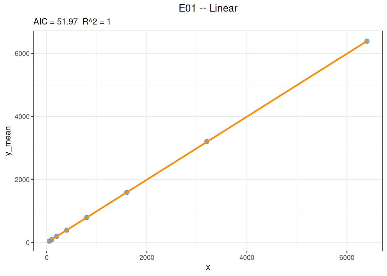

Code

predict(
  fit_lin,
  newdata = data.frame(x = c(0.5, 2, 8)),
  interval = "confidence"
)

   x        y  y_ci_lwr  y_ci_upr
 0.5 1.474737 -3.922223  6.871698
 2.0 2.973078 -2.421993  8.368150
 8.0 8.966442  3.578916 14.353968

Back-calculate concentration from response:

Code

predict(
  fit_lin,
  newdata = data.frame(y_mean = c(650, 3300, 6500)),
  inverse = TRUE
)

         x    y
  649.7434  650
 3302.6777 3300
 6506.2210 6500

Prediction boundaries: Inverse back-calculation should avoid extrapolating beyond the calibration concentration range. Linear back-calculation within range is stable, but in plateau or nonlinear regions, inverse prediction is very sensitive to response error.

6.4 Example 2: Polynomial Analysis of a Twofold Dilution

6.4.1 Reading and Validating Data

The data are 5 concentration levels × 3 replicates:

Code

poly_data <- read_csv("./data/linearity-polynomial.csv", show_col_types = FALSE)
poly_data <- as.data.frame(poly_data)
head(poly_data, 6)

6.4.2 Compute replicate means and introduce weights:

Code

rep_sum_w <- replicate_to_mean(
  poly_data,
  x = "conc",
  y = "signal",
  weights = "1/sd^2"
)
rep_sum_w

Parameter notes: The weights of replicate_to_mean() can be NULL (no weight column generated), "n", "1/sd", or "1/sd^2" (inverse-variance weighting). Weights should be determined based on the actual variance structure of the replicates or the protocol.

6.4.3 Candidate Equation Comparison

EP06-A2 typically compares linear, quadratic, and cubic models to determine whether higher-order terms are needed and to compare the residual standard errors:

Code

fit_poly_lin <- fit_equation("E01", data = rep_sum_w, x = "x", y = "y_mean", weights = rep_sum_w$weights)
print(fit_poly_lin)

E01 (Linear)
Formula: a + b*x

Call:
  stats::lm(formula = frm, data = d, weights = weights)

Residuals:
      Min       1Q   Median       3Q      Max
    -20.993  -17.367   -5.447   16.760   27.047

Coefficients:
   Estimate Std. Error  t value   Pr(>|t|)    
a -18.00771 20.0633790 -0.89754    0.43557    
b   1.01397  0.0188681 53.73983 1.4192e-05 ***
---
Signif. codes:  0 '***' 0.001 '**' 0.01 '*' 0.05 '.' 0.1 ' ' 1

Residual standard error: 24.3886 on 3 degrees of freedom
Multiple R-squared: 0.9990,  Adjusted R-squared: 0.9986
F-statistic: 2887.97 on 1 and 3 DF,  p-value: 1.42e-05

Code

fit_poly_qua <- fit_equation("E02", data = rep_sum_w, x = "x", y = "y_mean", weights = rep_sum_w$weights)
print(fit_poly_qua)

E02 (Quadratic)
Formula: a + b*x + c*x^2

Call:
  stats::lm(formula = frm, data = d, weights = weights)

Residuals:
      Min       1Q   Median       3Q      Max
    -13.443  -13.294  -13.146    8.912   30.970

Coefficients:
      Estimate  Std. Error t value  Pr(>|t|)   
a -7.14812e+00 3.09846e+01 -0.2307 0.8389994   
b  9.72049e-01 8.28550e-02 11.7319 0.0071872 **
c  2.34851e-05 4.48020e-05  0.5242 0.6524439   
---
Signif. codes:  0 '***' 0.001 '**' 0.01 '*' 0.05 '.' 0.1 ' ' 1

Residual standard error: 28.0077 on 2 degrees of freedom
Multiple R-squared: 0.9991,  Adjusted R-squared: 0.9982
F-statistic: 1095.05 on 2 and 2 DF,  p-value: 0.000912

Code

fit_poly_cub <- fit_equation("E12", data = rep_sum_w, x = "x", y = "y_mean", weights = rep_sum_w$weights)
print(fit_poly_cub)

E12 (Cubic)
Formula: a + b*x + c*x^2 + d*x^3

Call:
  stats::lm(formula = frm, data = d, weights = weights)

Residuals:
      Min       1Q   Median       3Q      Max
    -13.146   -2.191   -2.191    8.764    8.764

Coefficients:
      Estimate  Std. Error  t value Pr(>|t|)
a  2.04822e+01 2.48863e+01  0.82303  0.56161
b  7.25244e-01 1.39796e-01  5.18788  0.12123
c  3.86253e-04 1.91646e-04  2.01544  0.29321
d -1.35487e-07 7.07339e-08 -1.91545  0.30631

Residual standard error: 18.3308 on 1 degrees of freedom
Multiple R-squared: 0.9998,  Adjusted R-squared: 0.9992
F-statistic: 1705.48 on 3 and 1 DF,  p-value: 0.0178

6.5 Key Points for Interpreting Results

Separate fit from model judgment: A model being successfully fitted does not mean it is appropriate; judge in light of residuals, bias, acceptance criteria, and the protocol.
Residuals on two scales: Examine both original and relative residuals; for data spanning orders of magnitude, focus on relative residuals.
Weight rationale: Prefer the variance structure of the replicates or protocol requirements.
Range and extrapolation: Conclusions are valid only within the validated concentration range; avoid inverse prediction in plateau regions or beyond range.
Reproducibility: Save the raw data, code, model parameters, convergence information, package version, and complete session information.