5 Precision Analysis

5.1 Analysis Objectives

Precision evaluates the degree of agreement among results measured on the same sample by the same measurement system under repeatable conditions, usually expressed as the standard deviation (SD) or coefficient of variation (CV%). CLSI EP05 subdivides precision into variance components by condition, such as within-run, between-run, and between-day, and provides estimates, confidence intervals, and acceptance limits for judging each component.

This document demonstrates how to use the precision() function in the ivdtools package to establish a precision variance-component analysis, complete outlier checking, normality assessment, estimation of variance components and confidence intervals, Sadler precision profile fitting, and rearrangement of the results into an EP05-style variance component table. The example data are deterministic teaching data used only to demonstrate the analysis workflow; formal studies must use the experimental design, acceptance criteria, and analysis parameters pre-specified in the protocol or standard.

Code

library(ivdtools)
library(readr)

Data format requirement: precision() ultimately calls VCA::anovaVCA(), which requires a plain data.frame. Since readr::read_csv() reads in a tibble, this document consistently converts to a data.frame first, then converts the experimental factor columns (day, run, replicate, etc.) to factors.

5.2 Overview of Functions

Function	Main purpose	Key input or output
`precision()`	Create a precision variance-component analysis object	Nested formula, `by` grouping, balance check
`outlier()`	Per-sample outlier detection	Grubbs or IQR method
`normal()`	Per-sample normality test	Shapiro-Wilk etc., `level` controls the confidence level
`variance()` / `vc()`	Estimate variance components	VC, %Total, SD, CV%, `NegVC` passed here
`ci()`	Confidence intervals for SD/CV of each component	Satterthwaite approximation
`profile()`	Sadler precision profile fitting	10 candidate models, AIC selection
`list_sadler()`	View the 10 Sadler models	Model formula and type
`summary()` / `plot()`	Summarize and plot	`plot(type=...)` selects the graphic

After precision() creates the object, analysis results accumulate into the object step by step through outlier(), normal(), variance(), ci(), and profile(), and must be reassigned:

precision() -> outlier() -> normal() -> variance() -> ci() -> profile()

Only analyses that have been executed appear in summary(), and some plot() graphics depend on prior analyses.

5.3 Example 1: EP05 20×2×2 Single-Sample Precision

5.3.1 Reading and Validating Data

20×2×2 means 20 days, 2 runs per day, and 2 replicates per run, for a total of 80 results; it is one of the classic EP05 designs:

Code

ep05 <- read_csv("./data/precision-ep05.csv", show_col_types = FALSE)
ep05 <- as.data.frame(ep05)
str(ep05)

'data.frame':   80 obs. of  4 variables:
 $ day  : num  1 1 1 1 2 2 2 2 3 3 ...
 $ run  : num  1 1 2 2 1 1 2 2 1 1 ...
 $ rep  : num  1 2 1 2 1 2 1 2 1 2 ...
 $ value: num  96.9 93.5 99.3 101.5 103 ...

The experimental factor columns are integers in the CSV and are converted to factors after reading:

Code

ep05$day <- factor(ep05$day)
ep05$run <- factor(ep05$run)
ep05$rep <- factor(ep05$rep)

Code

dim(ep05)

[1] 80  4

Code

summary(ep05$value)

   Min. 1st Qu.  Median    Mean 3rd Qu.    Max. 
  86.06   94.83   99.33   99.11  103.53  115.01

value ~ day/run means the variance components are nested layer by layer as between-day (day) -> within-day run (run). / is the nesting notation, equivalent to treating each deeper factor as a factor nested within the factor above it.

5.3.2 Creating the Analysis Object and Pre-Check

Code

p <- precision(ep05, value ~ day/run)
p

Precision analysis object
  Data class          : data.frame
  Total rows          : 80
  Formula             : value ~ day/run
  Samples             : 1

Factor levels
  day         : 1 (4), 2 (4), 3 (4), 4 (4), 5 (4), 6 (4), 7 (4), 8 (4), 9 (4), 10 (4), 11 (4), 12 (4), 13 (4), 14 (4), 15 (4), 16 (4), 17 (4), 18 (4), 19 (4), 20 (4)
  run         : 1 (40), 2 (40)
  rep         : 1 (40), 2 (40)

Analysis status

  [ ] outlier
  [ ] normal
  [ ] variance
  [ ] ci
  [ ] profile

The balance check output reports the ratio of the largest to smallest cell size; when the data are highly unbalanced, VCA will suggest switching to REML.

Perform per-sample outlier detection and normality testing:

Code

p <- outlier(p, method = "grubbs")

Outlier detection -- Grubbs (alpha = 0.05)
  No outliers detected.

Code

p <- normal(p, method = "shapiro")

Normality test -- Shapiro-Wilk
  Sample               n           W  p-value
  ---------------------------------------------
  all                 80      0.9868  0.5858

Parameter notes: The method of outlier() can be "grubbs" (default) or "iqr", and alpha is the Grubbs significance level. For normal(), method="auto" selects the test based on sample size (Shapiro-Wilk for n≤50, Anderson-Darling for larger samples); when method="shapiro" is specified, the reported W column is the true Shapiro-Wilk W statistic. For single-sample data with n=80, either approach is acceptable; this example specifies it explicitly for illustration.

5.3.3 Variance Components and Confidence Intervals

Code

p <- variance(p)

Variance components
 sample component      VC %Total     SD  CV[%]
----------------------------------------------
    all       day 18.8358   42.6 4.3400 4.3788
    all   day:run 17.4343   39.4 4.1754 4.2128
    all     error  7.9482   18.0 2.8193 2.8445

The NegVC parameter needs to be passed at variance():

Code

p <- variance(p, NegVC = TRUE)   # allow negative variance components (default FALSE)

Code

p <- ci(p)

Confidence intervals (SD)
 sample component estimate  lower  upper
----------------------------------------
    all     total   6.6497 5.4288 8.5842
    all       day   4.3400 0.0000 6.2255
    all   day:run   4.1754 2.0129 5.5513
    all     error   2.8193 2.3147 3.6073 

Confidence intervals (%CV)
 sample component estimate  lower  upper
----------------------------------------
    all     total   6.7091 5.4773 8.6609
    all       day   4.3788 0.0000 6.2812
    all   day:run   4.2128 2.0309 5.6009
    all     error   2.8445 2.3353 3.6395

ci() uses the Satterthwaite effective-degrees-of-freedom approximation to compute confidence intervals for the SD and CV of each component.

5.3.4 Converting to an EP05 Terminology Table

Classify the variance components into within-run, between-run, and between-day by the nesting depth of the component name, compute the total SD/CV, and further merge the component confidence intervals to form a complete EP05 report table with intervals. Whether the statistical results are acceptable must be judged against the precision limits pre-specified in the protocol.

5.3.5 Graphics

A scatter plot can be used to quickly identify test anomalies and the distribution of measurements:

Code

plot(p, type = "dot")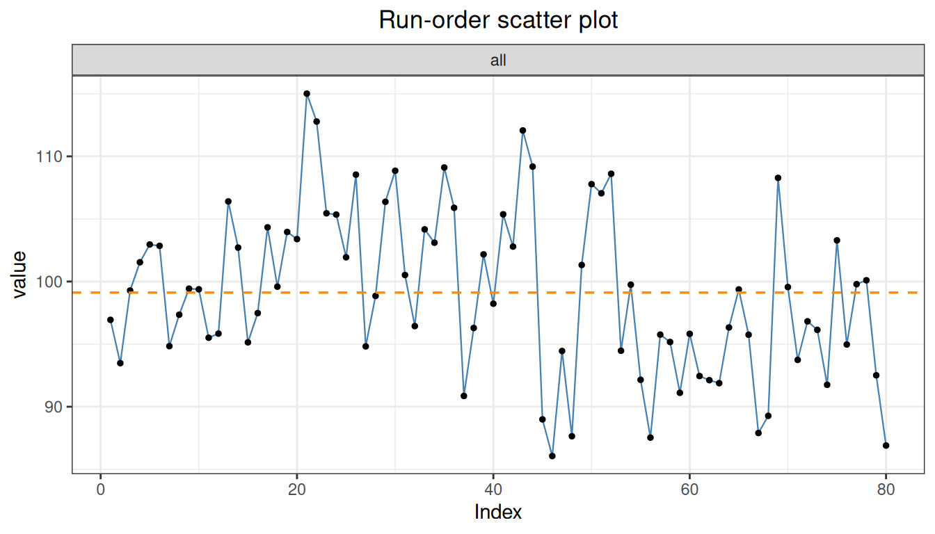

Code

plot(p, type = "qq")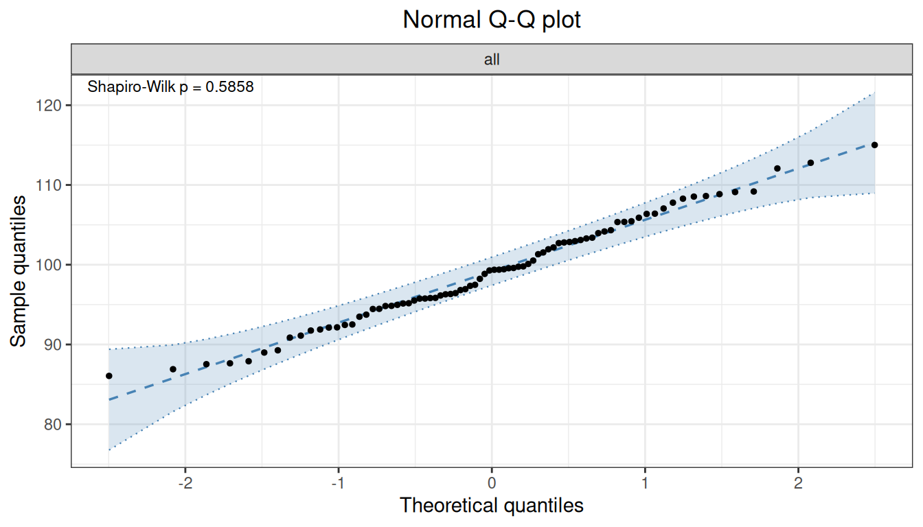

Graphic dependencies: plot(type="dot") is a scatter plot by run order (no prior analysis needed), type="his" is a standard histogram; type="var" requires variance() to have been run, type="qq" requires normal(), and type="profile" requires profile(). Confirm that the corresponding analysis has been run before plotting.

Code

summary(p)


Precision analysis -- summary
---------------------------------------- 

Precision analysis object
  Data class          : data.frame
  Total rows          : 80
  Formula             : value ~ day/run
  Samples             : 1

Factor levels
  day         : 1 (4), 2 (4), 3 (4), 4 (4), 5 (4), 6 (4), 7 (4), 8 (4), 9 (4), 10 (4), 11 (4), 12 (4), 13 (4), 14 (4), 15 (4), 16 (4), 17 (4), 18 (4), 19 (4), 20 (4)
  run         : 1 (40), 2 (40)
  rep         : 1 (40), 2 (40)

Analysis status

  [x] outlier
  [x] normal
  [x] variance
  [x] ci
  [ ] profile

Outlier detection -- Grubbs (alpha = 0.05)
  No outliers detected.

Normality test -- Shapiro-Wilk
  Sample               n           W  p-value
  ---------------------------------------------
  all                 80      0.9868  0.5858

Variance components
 sample component      VC %Total     SD  CV[%]
----------------------------------------------
    all       day 18.8358   42.6 4.3400 4.3788
    all   day:run 17.4343   39.4 4.1754 4.2128
    all     error  7.9482   18.0 2.8193 2.8445 

Confidence intervals (SD)
 sample component estimate  lower  upper
----------------------------------------
    all     total   6.6497 5.4288 8.5842
    all       day   4.3400 0.0000 6.2255
    all   day:run   4.1754 2.0129 5.5513
    all     error   2.8193 2.3147 3.6073 

Confidence intervals (%CV)
 sample component estimate  lower  upper
----------------------------------------
    all     total   6.7091 5.4773 8.6609
    all       day   4.3788 0.0000 6.2812
    all   day:run   4.2128 2.0309 5.6009
    all     error   2.8445 2.3353 3.6395

5.4 Example 2: Multi-Sample 3×5 and Sadler Profile

5.4.1 Reading Data

When multiple concentration levels need to be evaluated, use by to specify the sample grouping column, and estimate the variance components separately for each sample:

Code

profile_data <- as.data.frame(read_csv(
  "./data/precision-profile.csv",
  show_col_types = FALSE
))
profile_data$sample <- factor(profile_data$sample)
profile_data$day <- factor(profile_data$day)
profile_data$rep <- factor(profile_data$rep)

5.4.2 Per-Sample Variance Components

Code

p2 <- precision(profile_data, value ~ day, by = "sample")
p2 <- variance(p2)

Variance components
 sample component       VC %Total      SD  CV[%]
------------------------------------------------
     L1       day   0.6376   63.0  0.7985 3.9446
     L1     error   0.3750   37.0  0.6124 3.0250
     L2       day   5.7139   75.1  2.3904 4.7584
     L2     error   1.8937   24.9  1.3761 2.7393
     L3       day   3.3913   15.7  1.8415 1.8088
     L3     error  18.1466   84.3  4.2599 4.1840
     L4       day  30.5549   54.6  5.5276 2.7529
     L4     error  25.4525   45.4  5.0451 2.5126
     L5       day   0.0000    0.0  0.0000 0.0000
     L5     error 171.7986  100.0 13.1072 3.3003

Code

p2 <- ci(p2)

Confidence intervals (SD)
 sample component estimate  lower   upper
-----------------------------------------
     L1     total   1.0063 0.6007  2.9368
     L1       day   0.7985 0.0000  1.4267
     L1     error   0.6124 0.4391  1.0108
     L2     total   2.7582 1.5714  9.9889
     L2       day   2.3904 0.0000  4.2023
     L2     error   1.3761 0.9868  2.2716
     L3     total   4.6409 3.2872  7.8819
     L3       day   1.8415 0.0000  4.1779
     L3     error   4.2599 3.0547  7.0319
     L4     total   7.4838 4.6166 19.1652
     L4       day   5.5276 0.0000 10.0268
     L4     error   5.0451 3.6177  8.3280
     L5     total  13.1072 9.5629 20.8255
     L5       day   0.0000     NA      NA
     L5     error  13.1072 9.3990 21.6365 

Confidence intervals (%CV)
 sample component estimate  lower   upper
-----------------------------------------
     L1     total   4.9710 2.9673 14.5079
     L1       day   3.9446 0.0000  7.0480
     L1     error   3.0250 2.1692  4.9936
     L2     total   5.4905 3.1281 19.8843
     L2       day   4.7584 0.0000  8.3652
     L2     error   2.7393 1.9643  4.5219
     L3     total   4.5583 3.2287  7.7416
     L3       day   1.8088 0.0000  4.1035
     L3     error   4.1840 3.0003  6.9067
     L4     total   3.7271 2.2992  9.5447
     L4       day   2.7529 0.0000  4.9936
     L4     error   2.5126 1.8017  4.1476
     L5     total   3.3003 2.4078  5.2436
     L5       day   0.0000     NA      NA
     L5     error   3.3003 2.3666  5.4478

Comparing the proportion of variability across samples can be used for product optimization and testing scheme design:

Code

plot(p2, type = "var")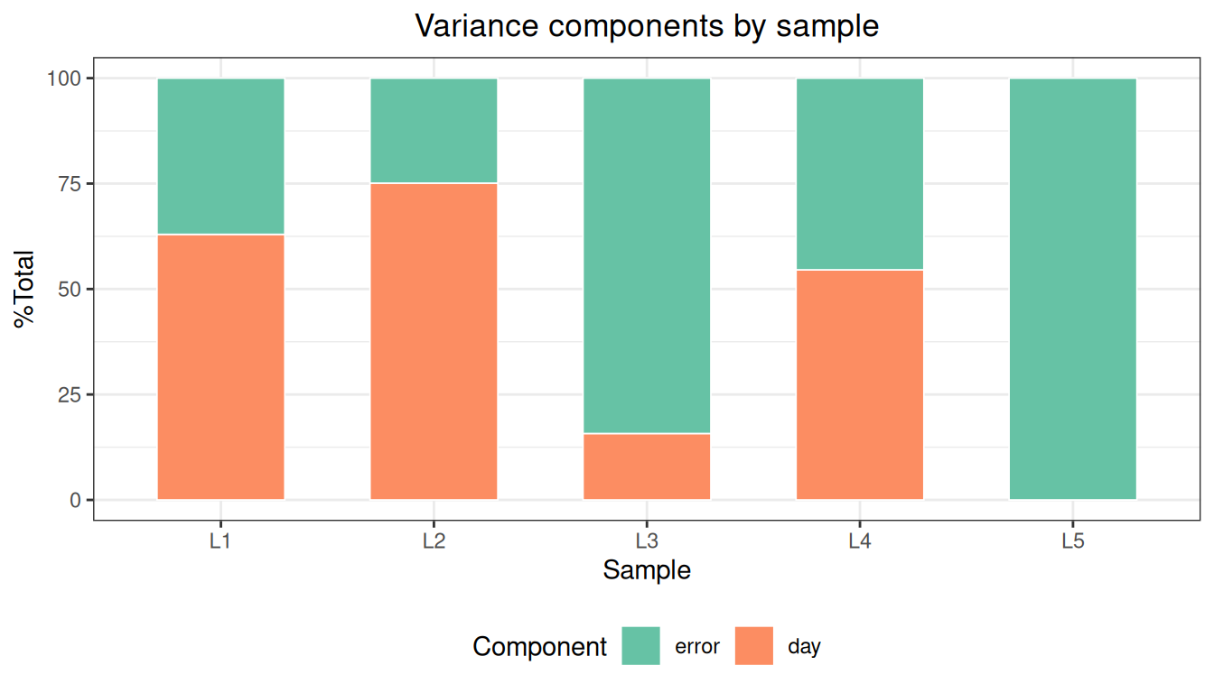

5.4.3 Precision Profile

profile() fits the Sadler model family to each variance component and selects the best model by AIC:

Code

list_sadler()

Sadler Precision Profile Models

   1  Constant SD           sigma^2 = b1
   2  Constant CV           sigma^2 = b1 * mu^2
   3  Linear (variance)     sigma^2 = b1 + b2 * mu
   4  Power (fixed K)       sigma^2 = b1 * mu^K
   5  Power (fixed K, +intercept)  sigma^2 = b1 + b2 * mu^K
   6  Linear (SD)           sigma = b1 + b2 * mu
   7  Power (SD)            sigma = b1 + b2 * mu^b3
   8  Power (variance)      sigma^2 = b1 + b2 * mu^b3
   9  Exponential (log-log)  log(sigma^2) = b1 + b2 * log(mu)
  10  Power (full)          sigma^2 = b1 * mu^b2

Code

p2 <- profile(p2, model.no = 1:10)

Precision profiles -- Sadler
  total: sigma = 0.0000 + 0.0086 * mu^1.6702  (AIC = 56.45, R^2 = 0.9847)
  day: sigma = 0.0000 + 0.0095 * mu^1.4951  (AIC = 43.46, R^2 = 0.8919)
  error: sigma^2 = 0.0010 * mu^2  (AIC = 55.96, R^2 = 0.9806)

Code

plot(p2, type = "profile")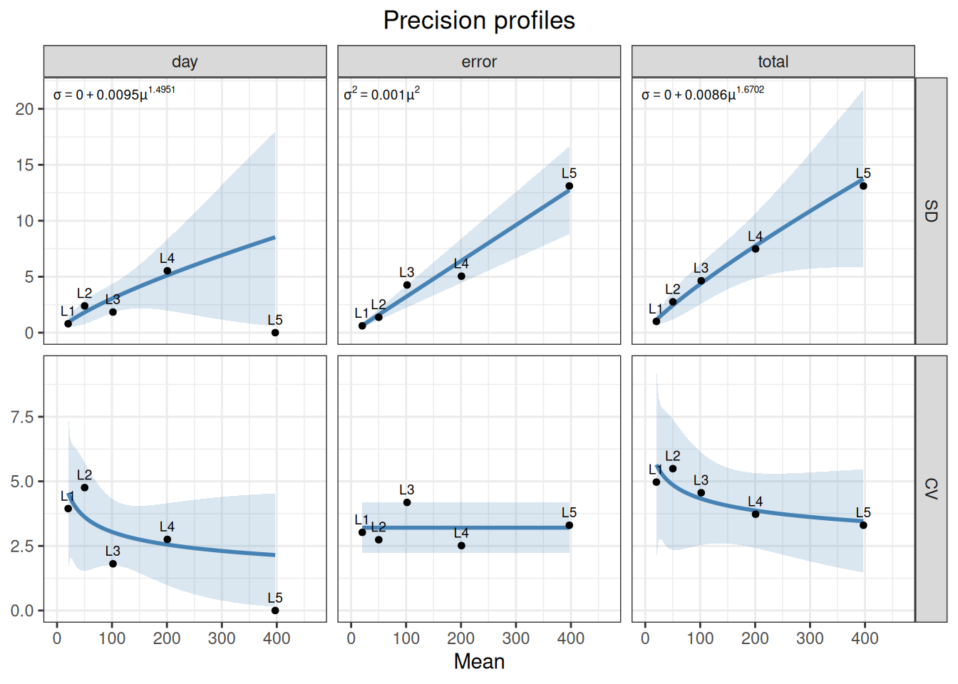

Parameter notes: profile(model.no = 1:10) specifies the candidate model numbers; ... can be passed to the internal Sadler fit (for example K). Each variance component requires at least 3 samples with a finite SD to be fitted, so a multi-sample design should include at least 3 concentration levels. The profile can be used, for example, in functional-sensitivity analyses to predict the SD/CV at any concentration (see 《Functional Sensitivity》).

In this example, the best models for the total and day components are power-function type (model 7), and the day:rep component is a constant-CV type (model 2), consistent with the common setting where “SD increases with concentration while CV is relatively stable”.

5.5 Example 3: Multi-Sample Multi-Site (Site) Precision

5.5.1 Reading Data

The data contain 2 sites, 3 samples, and per site per sample 3 days × 3 runs × 5 replicates:

Code

sites_data <- as.data.frame(read_csv(
  "./data/precision-sites.csv",
  show_col_types = FALSE
))
sites_data[] <- lapply(sites_data, function(x)
  if (is.numeric(x) && all(x == round(x))) factor(x) else x)
str(sites_data)

'data.frame':   270 obs. of  6 variables:
 $ site  : chr  "A" "A" "A" "A" ...
 $ sample: chr  "S1" "S1" "S1" "S1" ...
 $ day   : Factor w/ 3 levels "1","2","3": 1 1 1 1 1 1 1 1 1 1 ...
 $ run   : Factor w/ 3 levels "1","2","3": 1 1 1 1 1 2 2 2 2 2 ...
 $ rep   : Factor w/ 5 levels "1","2","3","4",..: 1 2 3 4 5 1 2 3 4 5 ...
 $ value : num  49.2 52.3 48.8 49.4 51.5 ...

5.5.2 Multi-Column Grouping

by can accept multiple column names and groups internally by the interaction, obtaining all site × sample combinations at once:

Code

p3 <- precision(sites_data, value ~ day/run, by = c("sample", "site"))
p3 <- variance(p3)

Variance components
 sample component      VC %Total     SD  CV[%]
----------------------------------------------
   S1.A       day  0.0000    0.0 0.0000 0.0000
   S1.A   day:run  0.1646    6.8 0.4057 0.8231
   S1.A     error  2.2677   93.2 1.5059 3.0553
   S2.A       day  0.3241    4.3 0.5693 0.5602
   S2.A   day:run  0.1523    2.0 0.3903 0.3840
   S2.A     error  7.0483   93.7 2.6549 2.6124
   S3.A       day  4.4871   15.6 2.1183 1.0420
   S3.A   day:run  1.7006    5.9 1.3041 0.6415
   S3.A     error 22.5797   78.5 4.7518 2.3375
   S1.B       day  0.0000    0.0 0.0000 0.0000
   S1.B   day:run  0.5459   23.5 0.7389 1.4758
   S1.B     error  1.7784   76.5 1.3335 2.6637
   S2.B       day  0.0000    0.0 0.0000 0.0000
   S2.B   day:run  1.6690   21.5 1.2919 1.2891
   S2.B     error  6.0856   78.5 2.4669 2.4616
   S3.B       day  0.7633    2.3 0.8737 0.4448
   S3.B   day:run  0.0000    0.0 0.0000 0.0000
   S3.B     error 31.8033   97.7 5.6394 2.8709

Code

names(p3$results)

[1] "S1.A" "S2.A" "S3.A" "S1.B" "S2.B" "S3.B"

5.5.3 Splitting by Site for Separate Analysis

An equivalent approach is to first split() by site and then run the same analysis parameters on each site subset. When the variance-component structure is expected to differ between sites, or separate reports are needed, splitting and analyzing separately is clearer:

Code

for (s in c("A", "B")) {
  sub <- sites_data[sites_data$site == s, ]
  ps <- precision(sub, value ~ day/run, by = "sample")
  ps <- variance(ps)
  ps <- ci(ps)
}

Note: Multi-center studies should unify the analysis plan, variance-component model, and reporting convention; when “reporting per center first and then combining”, be sure to record whether each center’s raw data were included, and whether the exclusion criteria and factor definitions are consistent.

5.6 Example 4: Custom More Complex Models

5.6.1 Reading Data

Besides the standard day/run/replicate nesting, the precision() formula can be any VCA nested structure, for example adding an operator level: value ~ operator/day/run, i.e., nested layer by layer as operator -> day -> run:

Code

custom_data <- as.data.frame(read_csv(
  "./data/precision-custom.csv",
  show_col_types = FALSE
))
custom_data[] <- lapply(custom_data, function(x)
  if (is.numeric(x) && all(x == round(x))) factor(x) else x)

5.6.2 Fitting and Interpretation

Code

p4 <- precision(custom_data, value ~ operator/day/run)
p4 <- variance(p4)

Variance components
 sample        component     VC %Total     SD  CV[%]
----------------------------------------------------
    all         operator 2.2914   11.8 1.5137 1.4898
    all     operator:day 6.3159   32.4 2.5132 2.4734
    all operator:day:run 3.2463   16.7 1.8017 1.7733
    all            error 7.6322   39.2 2.7627 2.7190

5.7 Key Points for Interpreting Results

Design match: First clarify the nesting structure of the study design; the precision() formula must faithfully reflect the experimental hierarchy.
Data format: After read_csv, convert to data.frame and explicitly convert factor columns to factor to avoid VCA errors or ambiguity.
Call order: outlier → normal → variance → ci → profile, reassign after each analysis; plotting depends on prior analyses.
Negative components: When a factor has too few levels or the data happen to be nearly identical, a variance component may be set to zero; interpret carefully and specify the handling approach in the protocol.
CI applicability: The Satterthwaite approximation becomes less accurate with very few variance components or unbalanced data; note the method in the report.
Terminology table: Rearrange the numeric quantities in $results (sd_comp/cv_comp/vc) into an EP05 terminology table; do not directly use the display-oriented string $vc.
Acceptability judgment: Statistical estimates do not automatically constitute a pass/fail determination; they should be compared with pre-specified precision limits and reviewed by professionals.