9 Reference Intervals

9.1 Analysis Objectives

A reference interval (RI) is defined by the measurement results of a reference sample population and is used to interpret the normal range of an individual’s results, corresponding to CLSI EP28-A3c. ivdtools provides three methods: the percentile method (nonparametric), the parametric method (normal or lognormal), and the robust method. The three methods differ in their sensitivity to sample size, distribution shape, and outliers; it is recommended to apply multiple methods to the same data simultaneously for comparison, and to perform outlier detection and normality assessment before establishing reference intervals.

This document demonstrates pre-analyses with outliers_test() and normal_test(), and then calls reference_interval(method = "all") to output the reference intervals of the three methods at once. The example data are deterministic teaching data (n=120, mildly right-skewed and containing outliers).

Code

library(ivdtools)
library(readr)

9.2 Overview of Functions

Function	Main purpose	Key input or output
`outliers_test()`	Outlier detection	Grubbs / ESD / Dixon / IQR
`normal_test()`	Normality test and graphics	`method="auto"` selects the test by sample size
`reference_interval()`	Reference intervals by three methods	`method="all"`, `interval`, `ci`, `id`
`plot.reference_interval()`	Plot intervals by method	jitter + upper/lower limits

9.3 Example: Reference Intervals Using Three Methods Together

9.3.1 Reading and Validating Data

Code

ri_data <- read_csv("./data/reference-interval.csv", show_col_types = FALSE)
ri_data <- as.data.frame(ri_data)
str(ri_data)

'data.frame':   120 obs. of  2 variables:
 $ id   : chr  "S001" "S002" "S003" "S004" ...
 $ value: num  131.1 100.8 106 74.3 116.9 ...

9.3.2 Pre-Analysis 1: Outlier Detection

EP28 recommends reviewing outliers before establishing reference intervals. With sample size n=120, Dixon is not suitable (Dixon applies only to n≤30), so use Grubbs and the generalized ESD:

Code

outliers_test(ri_data, col = "value", method = "grubbs")

Grubbs Outliers Test
  Data:   ri_data
  Column: value (n = 120, missing = 0)
  Parameters: alpha = 0.05
  Outliers: 1

  Index            Value      G stat    Critical
  -------------------------------------------
  88            183.0000      4.0104      3.4451

Code

outliers_test(ri_data, col = "value", method = "esd", r = 3)

Generalized ESD Outliers Test
  Data:   ri_data
  Column: value (n = 120, missing = 0)
  Parameters: alpha = 0.05, r = 3
  Outliers: 2

  Index            Value      R stat    Critical
  -------------------------------------------
  88            183.0000      4.0104      3.4451
  57            178.0000      4.0576      3.4424

Parameter notes: The method of outliers_test() can be "grubbs", "esd", "dixon", or "iqr"; ESD specifies the maximum number of detections via r, Dixon specifies the tail via type ("both"/"min"/"max"), and IQR specifies the multiplier via coef (default 1.5). Detecting an outlier does not mean it should be deleted — go back to the original records, experimental procedure, and protocol requirements, and perform an include/exclude sensitivity analysis when there is sufficient justification.

9.3.3 Pre-Analysis 2: Normality Test

Code

nt <- normal_test(ri_data, col = "value", method = "auto")
nt


Normality Test
  Data:   ri_data
  Column: value (n = 120, missing = 0)
  Method:     Anderson-Darling

  A = 1.7577, p = 0.0002

Code

plot(nt, type = c("qq", "his"))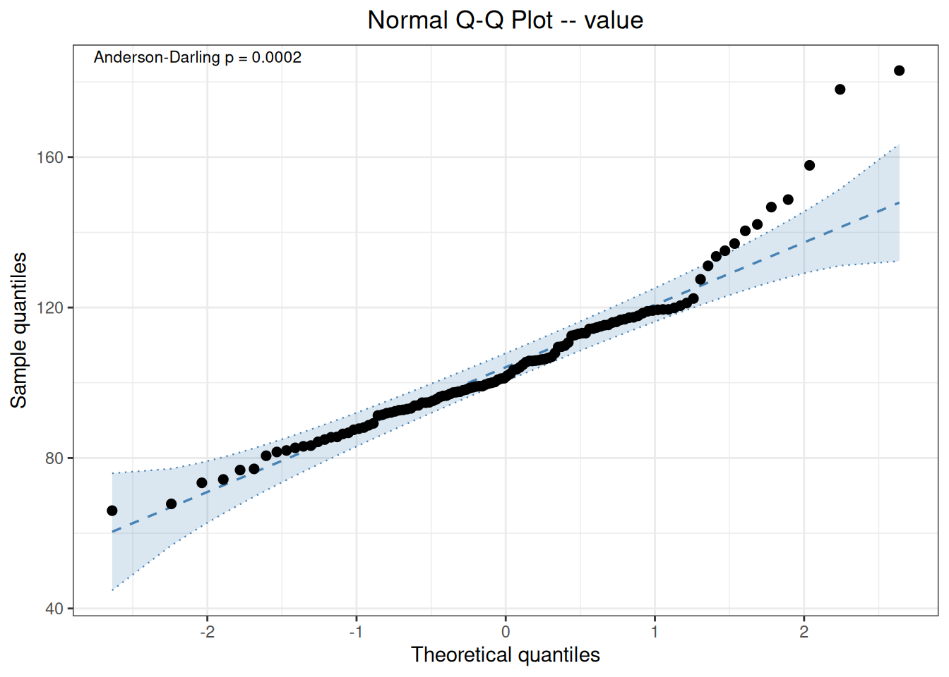

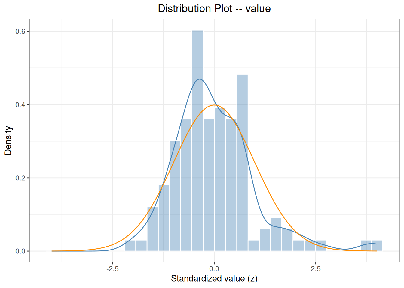
method="auto" automatically selects the Anderson-Darling test for n=120; the p-value is very small, indicating that the data do not follow a normal distribution (the data are right-skewed and contain outliers). The QQ plot and histogram can visually confirm the skewness.

9.3.4 Reference Intervals Using Three Methods Together

Code

ri <- reference_interval(
  ri_data,
  col = "value",
  interval = 0.95,
  ci = 0.95,
  method = "all",
  id = "id"
)
print(ri)


Reference Interval Analysis
  Column:              value
  Reference interval:  95% (alpha = 0.025)
  Confidence level:    0.95
  ID variable:         id
  Complete cases:      120 / 120

  No missing values.
  No duplicate IDs found.

  Percentile (quantile type 6, CLSI EP28-A3c)
    Lower = 73.4225  [66.0000, 80.6000]
    Upper = 157.5725  [137.0000, 183.0000]

  Parametric (log-transformed, Shapiro-Wilk p = 0.0661)
    Lower = 73.2539  [69.3807, 77.3434]
    Upper = 145.9407  [138.2241, 154.0880]

  Robust (Huber M-estimation (k=1.5, 16 iter) + MAD)
    Lower = 72.1573  [66.9058, 77.2532]
    Upper = 134.7365  [128.1754, 142.5643]

Code

pl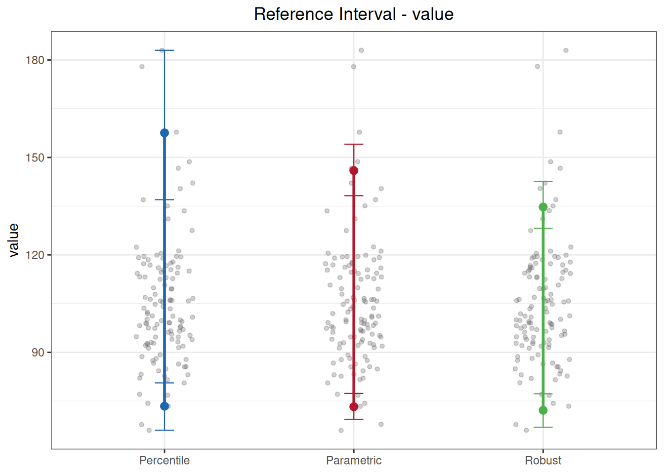ot(ri)

Parameter notes: In reference_interval(), interval is the coverage of the reference interval (default 0.95, corresponding to 2.5%–97.5%), while ci is the confidence level of the interval endpoints; the two have different meanings. method can be "percentile", "parametric", "robust", "all", or any combination of these. id is used for duplicate-sample detection.

Comparison of the three methods in this example:

Percentile method (73.4–157.6): nonparametric and makes no distributional assumption, but the upper limit is raised by two large outliers;
Parametric method (73.3–145.9): automatically detects non-normality and applies a log transformation (transformed=TRUE) before back-transforming;
Robust method (72.2–134.7): based on the Huber M-estimator and MAD, most robust to outliers.

The upper limit of the percentile method is clearly higher than that of the robust method, which is precisely the effect of the outliers. The reporting method should be selected under the guidance of the sample source, sample size, distribution characteristics, and study protocol, rather than simply picking the one whose result “looks best”.

9.4 Key Points for Interpreting Results

Protocol first: Specify the reference population, inclusion/exclusion criteria, sample size (EP28 recommends ≥120 for the percentile method), and partitioning strategy.
Check before compute: Perform outlier detection and normality assessment first, and record the outlier-handling decision (whether to exclude, and the basis).
Methods comparable: Outputting the three methods together helps reveal the effect of outliers or distributional assumptions on the interval; state the chosen method and its rationale in the report.
Distinguish parameters: Distinguish interval (coverage) from ci (endpoint confidence); do not mix them up.
Transparent transformation: When the parametric method automatically applies a log transformation, report the transformation type and the back-transformation method.
Non-unique conclusion: A reference interval is not the same as a clinical decision limit, nor does it automatically constitute an acceptability determination.