7  Analytical Sensitivity

7.1 Analysis Objectives

Analytical sensitivity describes the ability of a measurement system to distinguish “signal from noise” at the low-concentration end, and consists of three progressively increasing limits:

• LoB (Limit of Blank): The highest measurement that blank samples may produce (95th percentile).
• LoD (Limit of Detection): The lowest concentration that can be distinguished from blank at a 95% confidence level.
• LoQ (Limit of Quantitation): The lowest concentration at which the measurement result reaches a pre-specified precision target (for example CV = 20%).

This document demonstrates how to compute analytical sensitivity with the lob_lod_loq() function of the ivdtools package according to CLSI EP17-A2:

• LoB by the 5.3.3.1 parametric method: LoB = M_B + cp·SD_B, pooling all blank results into one pool, with cp = 1.645/√(1 − 1/(4(B−K))) the small-sample-adjusted 95% one-sided quantile (B is the total number of blank results, K the number of blank samples).
• LoD by 5.4.3: first fit a Sadler precision profile model (variance as a function of concentration) to the non-blank low-concentration samples, then perform fixed-point iteration from LoB, X = LoB + cp·SD_WL(X), with cp = 1.645/√(1 − 1/(4(N_TOT−K))).
• LoQ by Appendix D1 Example 1 (functional sensitivity): find the intersection of the precision profile with the target CV level line, √Var(X)/X = target_cv. This LoQ reflects only precision and does not include bias.

The example data are deterministic teaching data used only to demonstrate the workflow; formal studies must use the experimental design, target concentration, and acceptance criteria pre-specified in the protocol or standard.

library(ivdtools)
library(readr)

7.2 Overview of Functions

Function	Main purpose	Key input or output
lob_lod_loq()	Compute LoB / LoD / LoQ in one call	Summarized data, blank sample names, target CV
replicate_to_mean()	Summarize replicate measurements	Mean, SD, replicate count n
fit_equation()	Fit the Sadler precision profile (called internally)	eq="sadler", df_col
print() / plot()	Result display	Tabular summary, SD/CV dual panels

The input to lob_lod_loq() is an already summarized data.frame: one row per sample, containing a sample-name column, a mean column (i.e., concentration), an SD column, and a replicate-count n column; the column names can be freely specified. It internally and automatically completes the optimal Sadler model fitting, so no manual fitting is required.

7.3 Example: LoB / LoD / LoQ Analysis

7.3.1 Reading and Validating Data

The data contain 2 blank samples (blank_A, blank_B) and 6 low-concentration samples (L1–L6), each with replicate measurements (40 for each blank, 30 for each low concentration), for a total of 260 rows. The SD increases with concentration, consistent with the common low-end situation of “variance increasing with the mean”:

sens <- read_csv("./data/sensitivity.csv", show_col_types = FALSE)
sens <- as.data.frame(sens)
str(sens)

'data.frame':   260 obs. of  2 variables:
 $ sample: chr  "blank_A" "blank_A" "blank_A" "blank_A" ...
 $ value : num  0.024 -0.006 0.055 -0.072 0.057 -0.023 -0.05 0.003 0.051 0.029 ...

dim(sens)

[1] 260   2

table(sens$sample)

blank_A blank_B      L1      L2      L3      L4      L5      L6 
     40      40      30      30      30      30      30      30 

7.3.2 Per-Sample Summarization

Use replicate_to_mean() to group by sample name and compute the mean, SD, and replicate count (when the grouping variable is character, the original values are retained, so each blank occupies one row):

rep <- replicate_to_mean(data.frame(x = sens$sample, y = sens$value),
                         x = "x", y = "y")
rep$sample <- rep$x
rep$mean   <- rep$y_mean
rep$sd     <- rep$y_sd
rep$n      <- rep$y_n
rep[c("sample", "mean", "sd", "n")]

Note: lob_lod_loq() requires the variance model response to be the variance and weighted by degrees of freedom, so after summarizing you also need to add the two columns var = sd^2 and df = n − 1 to each row before passing them to lob_lod_loq(). If your data already contain these two columns, this step is unnecessary.

7.3.3 Computing LoB / LoD / LoQ

The blank parameter specifies the blank sample names (multiple allowed), and target_cv specifies the precision target for LoQ:

summ <- rep[c("sample", "mean", "sd", "n")]
res <- lob_lod_loq(summ, sample_col = "sample", mean_col = "mean",
                   sd_col = "sd", n_col = "n",
                   blank = c("blank_A", "blank_B"), target_cv = 0.20)
res

Limit of Blank / Detection / Quantitation (EP17-A2)
Precision profile: Sadler; best model = Model_3
  Equation            : sigma^2 = b1 + b2 * mu^2
  Parameters          : b1 = 0.010196, b2 = 0.010388
  Fit                 : AIC = -479.4; RSS = 0.08315; GoF p = 0.9437
  LoB  (parametric, B = 80, K = 2) : 0.08357
  LoD  (fixed-point)                : 0.2552
  LoQ  (CV = 20%)                    : 0.5868
Note: LoQ is based on precision ONLY; bias is not included.

Interpreting the results:

• LoB = 0.0836: the 95th percentile of blank measurements (parametric method), pooling B = 80 blank results and K = 2 blank samples.
• LoD = 0.26: the fixed point of X = LoB + cp·SD(X) on the precision profile, i.e., measurements above this concentration can be judged “non-blank”.
• LoQ = 0.59 (CV = 20%): the lowest concentration needed to reach the 20% precision target, based only on precision.

7.3.4 Returned Object Structure

lob_lod_loq() returns a sensitivity object, with each limit and parameter stored as a named component:

str(res, max.level = 1)

List of 13
 $ call     : language lob_lod_loq(data = summ, sample_col = "sample", mean_col = "mean", sd_col = "sd",      n_col = "n", blank = c("bl| __truncated__
 $ lob      : num 0.0836
 $ lod      : num 0.255
 $ loq      : num 0.587
 $ n_blank  : int 80
 $ B        : int 80
 $ K        : int 2
 $ target_cv: num 0.2
 $ cp_lob   : num 1.65
 $ cp_lod   : num 1.65
 $ fit      :List of 12
  ..- attr(*, "class")= chr "fit_equation"
 $ model    : chr "Model_3"
 $ notes    : chr(0) 
 - attr(*, "class")= chr "sensitivity"

res$lob

[1] 0.0835705

res$lod

[1] 0.2552205

res$loq

[1] 0.5867594

res$B

[1] 80

res$K

[1] 2

res$cp_lob

[1] 1.647643

res$cp_lod

[1] 1.646183

res$model

[1] "Model_3"

cp_lob and cp_lod are the two small-sample correction factors of EP17; model is the optimal Sadler model selected by AIC (in this example, model 3, the mixed-variance type).

7.3.5 Graphics

plot() draws the two precision-profile panels for SD and CV, overlays the LoB / LoD / LoQ reference lines, and visually shows the geometric meaning of each limit:

plot(res)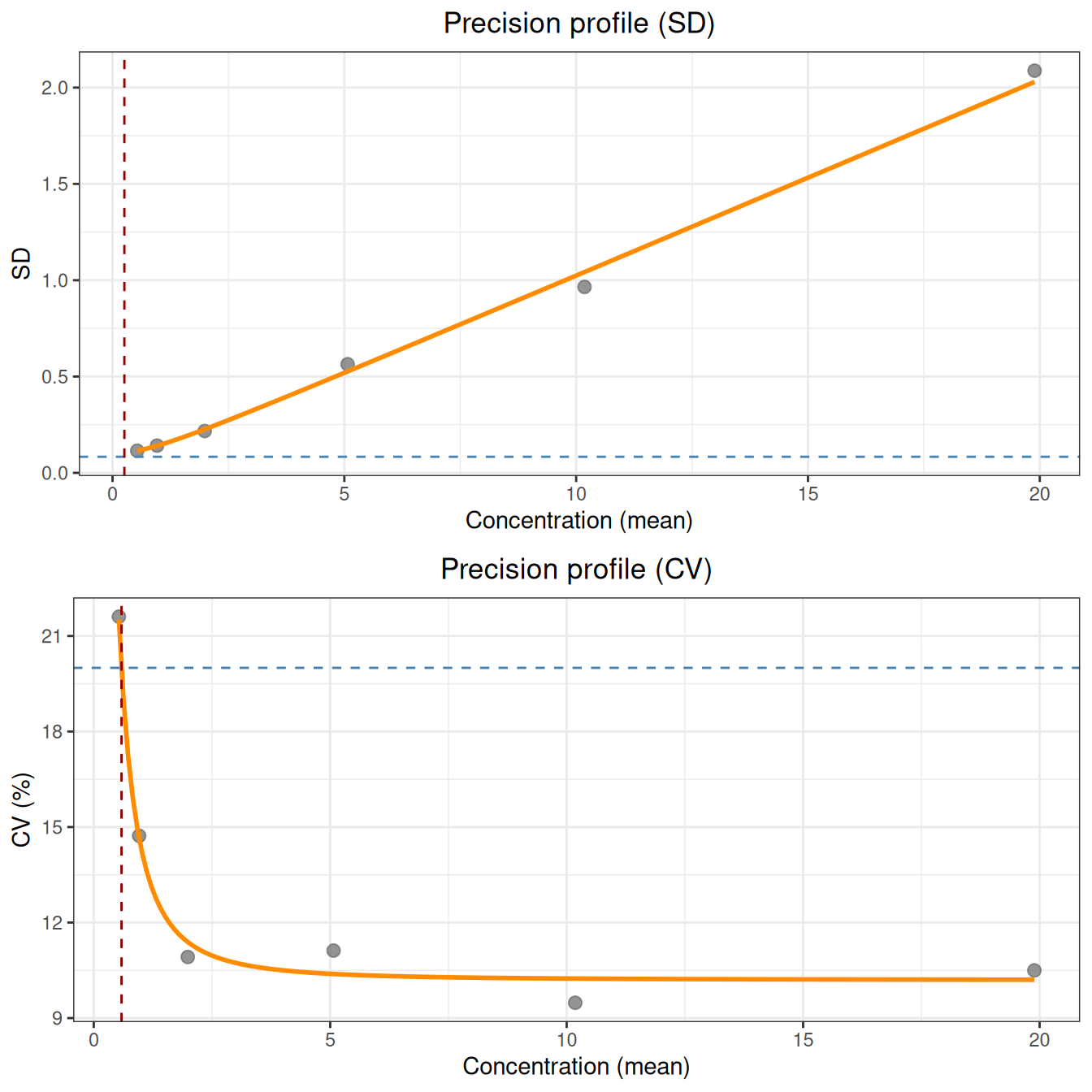

7.4 Other Input Scenarios

7.4.1 Scenario 1: Blank Only (LoB Only)

If there are no low-concentration levels, only LoB is computed, and LoD / LoQ are NA:

res_b <- lob_lod_loq(summ[summ$sample %in% c("blank_A", "blank_B"), ],
                     sample_col = "sample", mean_col = "mean",
                     sd_col = "sd", n_col = "n",
                     blank = c("blank_A", "blank_B"))
res_b

Limit of Blank / Detection / Quantitation (EP17-A2)
  LoB  (parametric, B = 80, K = 2) : 0.08357
  LoD  (fixed-point)                : --
  LoQ  (CV = 20%)                    : --
Note: LoQ is based on precision ONLY; bias is not included.

7.4.2 Scenario 2: No Blank (LoQ Only)

If there are no blank samples (blank = NULL), only LoQ is computed, and LoB / LoD are NA:

res_q <- lob_lod_loq(summ[!summ$sample %in% c("blank_A", "blank_B"), ],
                     sample_col = "sample", mean_col = "mean",
                     sd_col = "sd", n_col = "n")
res_q

Limit of Blank / Detection / Quantitation (EP17-A2)
Precision profile: Sadler; best model = Model_3
  Equation            : sigma^2 = b1 + b2 * mu^2
  Parameters          : b1 = 0.010196, b2 = 0.010388
  Fit                 : AIC = -479.4; RSS = 0.08315; GoF p = 0.9437
  LoB  (parametric, B = 0, K = 0) : --
  LoD  (fixed-point)                : --
  LoQ  (CV = 20%)                    : 0.5868
Note: LoQ is based on precision ONLY; bias is not included.

7.4.3 Scenario 3: LoQ < LoD

When the LoQ computed from the target CV is below the LoD (for example, large blank noise but good precision at low concentrations), LoQ takes max(LoQ, LoD) and issues a warning, ensuring LoQ ≥ LoD:

# Construct data with "large blank noise but good low-concentration precision"
d_noisy <- data.frame(
  sample = c("blank", paste0("L", 1:6)),
  mean   = c(0, 0.5, 1, 2, 5, 10, 20),
  sd     = c(5, sqrt(0.01 + 0.02 * c(0.5, 1, 2, 5, 10, 20)^2)),
  n      = c(30L, rep(5L, 6))
)
res_n <- lob_lod_loq(d_noisy, sample_col = "sample", mean_col = "mean",
                     sd_col = "sd", n_col = "n", blank = "blank")
res_n

Limit of Blank / Detection / Quantitation (EP17-A2)
Precision profile: Sadler; best model = Model_3
  Equation            : sigma^2 = b1 + b2 * mu^2
  Parameters          : b1 =   0.01, b2 =   0.02
  Fit                 : AIC = -469.2; RSS = 2.924e-29; GoF p =     1
  LoB  (parametric, B = 30, K = 1) : 8.261
  LoD  (fixed-point)                : 10.79
  LoQ  (CV = 20%)                    : 10.79
Note: LoQ is based on precision ONLY; bias is not included.
  Note: LoQ (precision) < LoD; LoQ reported as LoD = 10.79.

7.5 Key Points for Interpreting Results

1. Target first: Before analysis, determine the target CV (20% in this document is only a teaching example), confidence level, and acceptance criteria.
2. Blank pooled pool: LoB pools all blank results for computation; cp includes a B−K degrees-of-freedom correction that cannot be ignored when the sample size is small.
3. LoQ contains only precision: With this workflow, LoQ does not include bias and cannot replace a total-error (TE)-based limit-of-quantitation claim.
4. Model selection: Different Sadler models extrapolate very differently at the low-concentration end; the report should note the AIC-optimal model and its ranking.
5. LoQ ≥ LoD: The program guarantees LoQ is not below LoD; if the CV-based LoQ is below the LoD, it warns and takes max.
6. Data format: The input to lob_lod_loq() is an already-summarized data.frame; the original replicate data must first be processed by replicate_to_mean().