3 4PLC Equation Calibration Curve Fitting

3.1 Analysis Objectives

This document demonstrates how to fit a four-parameter logistic (4PLC) calibration curve using fit_equation() from the ivdtools package, and how to examine convergence status, residuals, weight effects, and forward and inverse prediction.

4PLC is a nonlinear model. A successfully returned fit object does not imply the model is adequate; formal analysis should also incorporate the calibration point design, lower and upper asymptote coverage, parameter stability, residual structure, repeat-measurement precision, and pre-specified acceptance criteria.

Code

library(ivdtools)
library(readr)

3.2 4PLC Model and Main Functions

In ivdtools, 4PLC corresponds to E07 and can also be invoked by the name "4PLC":

\[y = A + \frac{B-A}{1 + (x/C)^D}\]

Here, \(A\) and \(B\) denote the two asymptotic plateaus, \(C\) denotes the concentration scale at the curve midpoint, and \(D\) controls the curve direction and steepness. The meaning of the parameters should be interpreted in the context of the actual signal direction.

Function	Purpose
`list_equation()`	View the built-in equation registry
`replicate_to_mean()`	Summarize replicate measurements and optionally compute weights
`fit_equation()`	Fit built-in or custom equations
`coef()`	Extract model parameters
`residuals()`	Extract residuals (observed minus fitted)
`predict()`	Forward prediction of response or inverse estimation of concentration
`plot()`	Plot observed points, fitted curve, and intervals
`compare_equation()`	Compare candidate equations

View the response-curve models:

Code

list_equation(category = "Response")

  ID       Name                         Formula        Params nP Engine
-----------------------------------------------------------------------
 E01     Linear                         a + b*x          a, b  2     lm
 E02  Quadratic                 a + b*x + c*x^2       a, b, c  3     lm
 E03 ExpoGrowth                  a * exp(b * x)          a, b  2    nls
 E04  ExpoDecay                 a * exp(-b * x)          a, b  2    nls
 E05      Power                         a * x^b          a, b  2    nls
 E06        Log                  a + b * log(x)          a, b  2     lm
 E07       4PLC   A + (B - A) / (1 + (x / C)^D)    A, B, C, D  4    nls
 E08       5PLC A + (B - A) / (1 + (x / C)^D)^E A, B, C, D, E  5    nls
 E09   Gaussian a * exp(-(x - b)^2 / (2 * c^2))       a, b, c  3    nls
 E10  Michaelis             Vmax * x / (Km + x)      Vmax, Km  2    nls
 E11 Sinusoidal          a * sin(b * x + c) + d    a, b, c, d  4    nls
 E12      Cubic         a + b*x + c*x^2 + d*x^3    a, b, c, d  4     lm

fit_equation() can use automatic starting values or take them via start; lower, upper, and constraints set parameter bounds or constraints. weights accepts a numeric vector or the built-in schemes "equal", "1/y", "1/y^2", "1/x", "1/x^2".

Note: Weights should reflect the measurement error or variance structure; they should not be chosen only because the curve is positively or negatively correlated. It is best to pre-specify weights based on repeat-measurement precision, residual diagnostics, or the study protocol.

3.3 Example 1: Basic Fitting Workflow

3.3.1 Reading and Validating Data

Code

u1 <- read_csv("./data/4PLC-U1.csv", show_col_types = FALSE)
u1

Code

str(u1)

spc_tbl_ [6 × 3] (S3: spec_tbl_df/tbl_df/tbl/data.frame)
 $ Sample: chr [1:6] "s1" "s2" "s3" "s4" ...
 $ Con   : num [1:6] 0 4.08 24.93 92.75 338.54 ...
 $ RLU   : num [1:6] 1581 3857 12931 36153 106083 ...
 - attr(*, "spec")=
  .. cols(
  ..   Sample = col_character(),
  ..   Con = col_double(),
  ..   RLU = col_double()
  .. )
 - attr(*, "problems")=<externalptr>

Code

summary(u1[c("Con", "RLU")])

      Con                RLU        
 Min.   :   0.000   Min.   :  1581  
 1st Qu.:   9.293   1st Qu.:  6126  
 Median :  58.840   Median : 24542  
 Mean   : 246.308   Mean   : 77388  
 3rd Qu.: 277.092   3rd Qu.: 88600  
 Max.   :1017.550   Max.   :303726

Code

anyDuplicated(u1$Sample)

[1] 0

Code

sum(!is.finite(u1$Con) | !is.finite(u1$RLU))

[1] 0

This data contains 6 concentration levels. Because 4PLC requires estimating 4 parameters, the residual degrees of freedom are very few; in addition, the highest concentration does not yet clearly cover the upper plateau, so the model parameters may be unstable. This example is mainly intended to illustrate the operating workflow and should not be used directly as a formal calibration design example.

If each concentration contains replicates, you can fit all observations directly, or first summarize them with replicate_to_mean(). Whether to summarize and how to weight should be stated in the analysis plan.

3.3.2 Fitting and Checking Convergence

Code

fit_u1 <- fit_equation(
  "4PLC",
  data = u1,
  x = "Con",
  y = "RLU"
)
print(fit_u1)

E07 (4PLC)
Formula: A + (B - A) / (1 + (x / C)^D)

Call:
  fit_equation(eq = "4PLC", data = u1, x = "Con", y = "RLU")

Residuals:
      Min       1Q   Median       3Q      Max
    -1991.214  -1335.541  -252.849  960.620  2652.956

Coefficients:
      Estimate  Std. Error  t value Pr(>|t|)  
A  3.10445e+03 2.09875e+03  1.47919 0.277197  
B  6.13447e+07 2.60964e+09  0.02351 0.983380  
C  2.60778e+05 1.18118e+07  0.02208 0.984391  
D -9.58182e-01 1.20691e-01 -7.93917 0.015498 *
---
Signif. codes:  0 '***' 0.001 '**' 0.01 '*' 0.05 '.' 0.1 ' ' 1

Residual standard error: 2775.94 on 2 degrees of freedom
AIC: 115.58  Iterations: 50

Do not ignore the optimizer’s convergence information:

Code

fit_u1$fit$convInfo[c("isConv", "finIter", "stopCode", "stopMessage")]

$isConv
[1] FALSE

$finIter
[1] 50

$stopCode
[1] -1

$stopMessage
[1] "Number of iterations has reached `maxiter' == 50."

The default fit for this data reaches the iteration limit without declaring convergence. Increasing the maximum number of iterations sometimes helps, but cannot resolve a calibration range that does not cover a plateau or parameters that are not identifiable. When convergence is not achieved, inspect the data, model direction, starting values, parameter bounds, and calibration point design in turn, rather than accepting the result based only on the curve appearance.

3.3.3 Residuals and Graphics

Code

u1_diagnostics <- data.frame(
  Sample = u1$Sample,
  Con = u1$Con,
  RLU = u1$RLU,
  Residual = residuals(fit_u1),
  Relative_residual_pct = residuals(fit_u1) / u1$RLU * 100
)
knitr::kable(u1_diagnostics, digits = 2)

Sample	Con	RLU	Residual	Relative_residual_pct
s1	0.00	1581	-1523.45	-96.36
s2	4.08	3857	-771.83	-20.01
s3	24.93	12931	1192.12	9.22
s4	92.75	36153	2652.96	7.34
s5	338.54	106083	-1991.21	-1.88
s6	1017.55	303726	266.13	0.09

Code

plot(fit_u1, interval = "confidence", level = 0.95)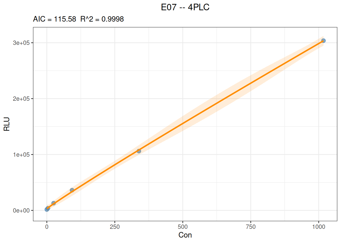

Residuals should be examined on both the original response scale and the relative scale, and interpreted together with the repeat-measurement variance. For responses spanning several orders of magnitude, looking at original residuals alone may let high-signal points dominate the judgment.

3.3.4 Predicting Response from Concentration

Code

predict(
  fit_u1,
  newdata = data.frame(Con = c(20, 200, 1000)),
  interval = "confidence",
  level = 0.95
)

    x         y   y_ci_lwr  y_ci_upr
   20  10095.70   5194.229  14997.17
  200  66540.68  59494.141  73587.22
 1000 298518.29 289967.527 307069.05

The mean confidence interval describes the uncertainty of the fitted mean; the prediction interval also includes single-observation error and is usually wider:

Code

predict(
  fit_u1,
  newdata = data.frame(Con = c(20, 200, 1000)),
  interval = "prediction",
  level = 0.95
)

    x         y      y_pi_lwr  y_pi_upr
   20  10095.70     -7.215948  20198.61
  200  66540.68  55240.318293  77841.05
 1000 298518.29 286223.575001 310813.01

3.3.5 Estimating Concentration from Response (Inverse Prediction)

Code

predict(
  fit_u1,
  newdata = data.frame(RLU = c(20000, 100000, 250000)),
  inverse = TRUE
)

        x      y
  50.2395  20000
 311.3672 100000
 828.5559 250000

Prediction boundaries: Avoid extrapolating beyond the calibration concentration range. Inverse prediction is very sensitive to response error in the plateau region, and non-monotonic models can also have multiple solutions. The current example fit did not converge reliably, so the predictions are used only to demonstrate the interface and cannot be used for quantitative conclusions.

3.4 Example 2: Sandwich Assay and Weights

3.4.1 Equal-Weight Fit

Sandwich assay data typically show increasing signal with increasing concentration. This example first performs an equal-weight fit:

Code

u2 <- read_csv("./data/4PLC-U2.csv", show_col_types = FALSE)

fit_u2_equal <- fit_equation(
  "4PLC",
  data = u2,
  x = "Con",
  y = "RLU"
)
print(fit_u2_equal)

E07 (4PLC)
Formula: A + (B - A) / (1 + (x / C)^D)

Call:
  fit_equation(eq = "4PLC", data = u2, x = "Con", y = "RLU")

Residuals:
      Min       1Q   Median       3Q      Max
    -1034493.852  -58331.509  17644.023  45830.410  785037.098

Coefficients:
      Estimate  Std. Error  t value   Pr(>|t|)    
A -4.19069e+04 2.74298e+05 -0.15278 0.88288329    
B  4.01980e+08 9.51404e+08  0.42251 0.68532695    
C  1.12895e+03 3.16059e+03  0.35720 0.73147078    
D -1.02539e+00 1.32241e-01 -7.75390 0.00011121 ***
---
Signif. codes:  0 '***' 0.001 '**' 0.01 '*' 0.05 '.' 0.1 ' ' 1

Residual standard error: 565331 on 7 degrees of freedom
AIC: 327.64  Iterations: 24

3.4.2 Inverse Response-Squared Weight Fit

When the response variance clearly increases with signal, an inverse-response-squared weight can be evaluated:

Code

fit_u2_weighted <- fit_equation(
  "4PLC",
  data = u2,
  x = "Con",
  y = "RLU",
  weights = "1/y^2"
)
print(fit_u2_weighted)

E07 (4PLC)
Formula: A + (B - A) / (1 + (x / C)^D)

Call:
  fit_equation(eq = "4PLC", data = u2, x = "Con", y = "RLU", weights = "1/y^2")

Residuals:
      Min       1Q   Median       3Q      Max
    -1038926.254  -2031.562  491.283  35707.649  809345.965

Coefficients:
      Estimate  Std. Error    t value   Pr(>|t|)    
A  5.66828e+03 2.30614e+02   24.57907 4.7016e-08 ***
B  2.00185e+08 6.72603e+07    2.97627   0.020624 *  
C  4.83741e+02 1.74222e+02    2.77658   0.027433 *  
D -1.08082e+00 1.02400e-02 -105.54858 1.8062e-12 ***
---
Signif. codes:  0 '***' 0.001 '**' 0.01 '*' 0.05 '.' 0.1 ' ' 1

Residual standard error: 0.042025 on 7 degrees of freedom
AIC: 265.29  Iterations: 7

Compare the relative residuals of the two models at each calibration point:

Code

u2_comparison <- data.frame(
  Sample = u2$Sample,
  Con = u2$Con,
  RLU = u2$RLU,
  Equal_weight_pct = residuals(fit_u2_equal) / u2$RLU * 100,
  Inverse_y2_weight_pct = residuals(fit_u2_weighted) / u2$RLU * 100
)
knitr::kable(u2_comparison, digits = 2)

Sample	Con	RLU	Equal_weight_pct	Inverse_y2_weight_pct
c1	0.00	5637	843.43	-0.55
c2	0.05	16014	275.49	3.07
c3	0.20	47520	67.84	-4.70
c4	0.51	125038	14.11	-1.46
c5	1.03	277621	4.57	4.70
c6	5.19	1498023	-4.39	0.98
c7	10.92	3334387	-1.53	1.70
c8	20.83	6148959	-6.53	-5.30
c9	49.90	16515788	4.75	4.13
c10	95.47	28504677	-3.63	-3.64
c11	112.18	35017203	1.75	2.31

Code

data.frame(
  Model = c("Equal weight", "1/y^2 weight"),
  Median_absolute_relative_residual_pct = c(
    median(abs(u2_comparison$Equal_weight_pct)),
    median(abs(u2_comparison$Inverse_y2_weight_pct))
  ),
  Maximum_absolute_relative_residual_pct = c(
    max(abs(u2_comparison$Equal_weight_pct)),
    max(abs(u2_comparison$Inverse_y2_weight_pct))
  )
) |>
  knitr::kable(digits = 2)

Model	Median_absolute_relative_residual_pct	Maximum_absolute_relative_residual_pct
Equal weight	4.75	843.43
1/y^2 weight	3.07	5.30

In this example data, the 1/y^2 weight clearly reduces the relative residuals at low-signal points; this only indicates that this weight better matches the relative-error evaluation objective adopted for this data. The formal choice still needs to combine the variance of the replicates at each concentration, the back-calculated concentration bias, model parameter stability, and pre-specified acceptance criteria. The residual standard errors and AIC under different weights have different scales and should not be compared directly without an error model.

Code

plot(fit_u2_weighted, interval = "confidence", level = 0.95)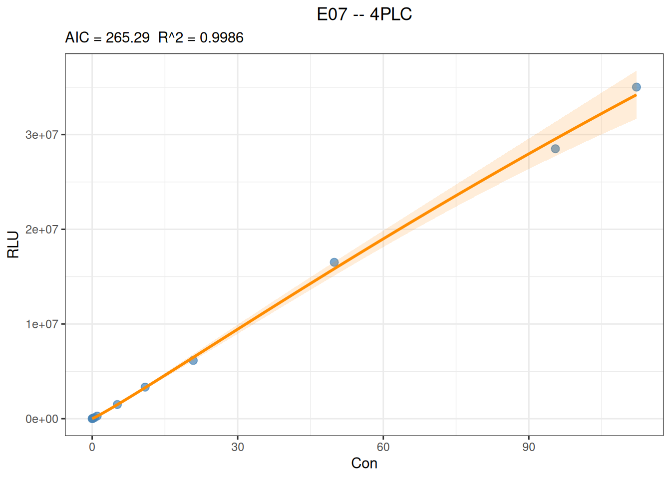

3.5 Example 3: Competitive Assay

Competitive assay data typically show decreasing signal with increasing concentration:

Code

u3 <- read_csv("./data/4PLC-U3.csv", show_col_types = FALSE)

fit_u3 <- fit_equation(
  "4PLC",
  data = u3,
  x = "Con",
  y = "RLU"
)
print(fit_u3)

E07 (4PLC)
Formula: A + (B - A) / (1 + (x / C)^D)

Call:
  fit_equation(eq = "4PLC", data = u3, x = "Con", y = "RLU")

Residuals:
      Min       1Q   Median       3Q      Max
    -1937.581  -454.210  -28.126  625.582  1807.765

Coefficients:
      Estimate  Std. Error   t value   Pr(>|t|)    
A -2.81576e+04 2.17005e+03  -12.9755 1.1793e-06 ***
B  1.40035e+06 1.08896e+03 1285.9562 < 2.22e-16 ***
C  1.29783e+02 6.49733e-01  199.7479 4.4162e-16 ***
D  7.82733e-01 2.79342e-03  280.2058 < 2.22e-16 ***
---
Signif. codes:  0 '***' 0.001 '**' 0.01 '*' 0.05 '.' 0.1 ' ' 1

Residual standard error: 1093.1 on 8 degrees of freedom
AIC: 207.11  Iterations: 5

Code

fit_u3$fit$convInfo[c("isConv", "finIter", "stopCode", "stopMessage")]

$isConv
[1] TRUE

$finIter
[1] 5

$stopCode
[1] 1

$stopMessage
[1] "Relative error in the sum of squares is at most `ftol'."

Code

u3_diagnostics <- data.frame(
  Sample = u3$Sample,
  Con = u3$Con,
  RLU = u3$RLU,
  Relative_residual_pct = residuals(fit_u3) / u3$RLU * 100
)
knitr::kable(u3_diagnostics, digits = 2)

Sample	Con	RLU	Relative_residual_pct
m1	0	1400548	0.01
m2	40	991716	-0.20
m3	60	897247	0.20
m4	79	822749	-0.05
m5	138	669646	0.11
m6	187	585293	0.10
m7	297	462119	-0.07
m8	523	330399	-0.19
m9	737	263095	-0.25
m10	1266	177260	-0.12
m11	1608	146827	0.11
m12	2218	112252	0.61

Code

plot(fit_u3, interval = "confidence", level = 0.95)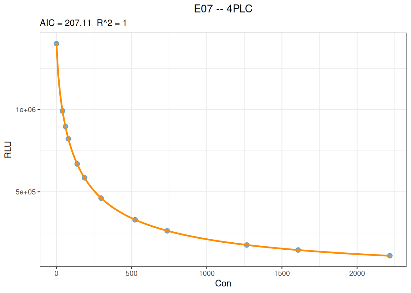

In this example, the equal-weight fit has already converged and the in-sample relative residuals are small, but you should still decide whether weights are needed based on the replicate measurement variance. The signal direction itself is not a basis for choosing between equal-weight and weighted fitting.

3.6 Key Points for Interpreting Results

Calibration design: Concentration points should cover the intended working range and, where possible, provide information about the upper and lower plateaus.
Convergence status: Check convInfo; do not treat reaching the maximum iterations as successful convergence.
Parameter plausibility: Judge stability in light of the plateaus, curve midpoint, direction, standard errors, and parameter correlations.
Residual structure: Examine the original residuals, relative residuals, and their variation with concentration or fitted value.
Weight rationale: Prefer variance structures estimated from replicate measurements, and specify the selection rule before analysis.
Back-calculation performance: Evaluate the back-calculated concentration bias and precision at each calibration point as required by the project.
Prediction range: Avoid extrapolation, especially unstable inverse prediction in the plateau region.
Reproducibility: Save the raw data, code, model parameters, package version, figures, and complete session information.