2 Installing and Using the Analysis Environment

2.1 Purpose of This Document

This document explains how to set up the ivdtools analysis environment, create an R Markdown project, import and validate data, run a progressive analysis, and save reproducible results.

2.2 Installing R

ivdtools 0.1.1 requires R >= 4.1.0. It is recommended to use a still-supported newer R version and to keep the same major version and dependency versions across all people in the project.

2.2.1 Windows and macOS

Download the installer for your system from CRAN: https://cran.r-project.org/.

Windows: install R; Rtools of a matching version is needed only when building packages containing native code from source.
macOS: choose the installer according to your processor architecture; Xcode Command Line Tools may be needed when building from source.

2.2.2 Debian/Ubuntu

The base R can be installed from the system repository:

sudo apt update
sudo apt install r-base r-base-dev

2.2.3 Fedora

sudo dnf install R R-devel

The R version in Linux distribution repositories may be older; if the project needs a newer R, configure the software source according to the CRAN instructions for the corresponding distribution.

2.3 Choosing an Editor

It is recommended to use .Rmd or .qmd files to record code, text, tables, and figures.

Software	Windows	Linux	macOS	Suitable for
RStudio	✓	✓	✓	Works out of the box; suitable for beginners and routine analysis
Positron	✓	✓	✓	Suitable for users who want the new-generation Posit IDE
Visual Studio Code	✓	✓	✓	Requires configuring R, Quarto and other extensions
Jupyter	✓	✓	✓	Requires Python, Jupyter and an R kernel
PyCharm	✓	✓	✓	Requires corresponding R support and extra configuration

RStudio and Positron can be obtained from https://posit.co/downloads/; Visual Studio Code can be obtained from https://code.visualstudio.com/Download.

2.4 Installing R Packages

Once ivdtools has been released on the CRAN mirror you use:

Code

install.packages(c("ivdtools", "rmarkdown", "knitr"))

Additional packages can be installed as needed for data import:

Code

install.packages(c("readr", "readxl"))

2.5 Creating a New Project

In RStudio, choose File > New File > R Markdown.

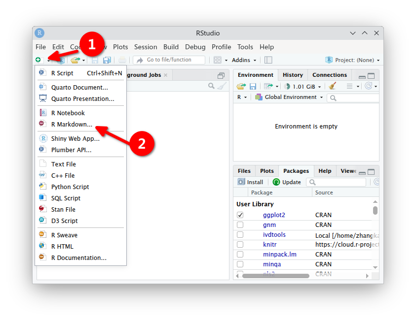
Minimal document template:

---
title: "IVD Analysis Report"
author: "Analyst"
date: "Enter the report date"
output:
  html_document:
    toc: true
    number_sections: true
---

Then insert an R code chunk named setup with include=FALSE set, containing the following:

knitr::opts_chunk$set(collapse = TRUE, comment = "#>")
library(ivdtools)

2.6 Importing and Validating Data

2.6.1 CSV

Base R:

Code

dat <- read.csv(
  "data-raw/method-comparison.csv",
  stringsAsFactors = FALSE,
  check.names = FALSE
)

Using readr:

Code

dat <- readr::read_csv(
  "data-raw/method-comparison.csv",
  show_col_types = FALSE
)

2.6.2 Excel

Code

dat <- readxl::read_excel(
  "data-raw/method-comparison.xlsx",
  sheet = "data"
)

If the Excel file contains formulas, merged cells, or manual formatting, first confirm that the imported values, column names, and data types match the original sheet.

2.7 Running Code

In a .Rmd, insert an R code chunk and use the button at the top-right of the chunk to run the current chunk, or run all code from top to bottom.

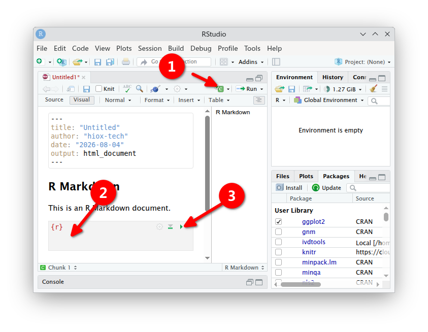
To ensure reproducibility, the final report should be rendered from scratch in a fresh R session, rather than relying on objects already present in the Console.

2.8 Exporting Results

2.8.1 Tables

After reading the result fields described on the help page, you can write out a CSV:

Code

# Example: the actual fields should be confirmed against the help page of the corresponding object
result_table <- mc$regression
saveRDS(result_table, "tables/regression-result.rds")

Complex objects are best saved as RDS to preserve their class and attributes; when exchanging with other software, tidy them into flat data frames and export as CSV.

2.8.2 Figures

Code

p <- plot(mc, type = "bland_altman")
ggplot2::ggsave(
  "figures/bland-altman.png",
  plot = p,
  width = 7,
  height = 5,
  dpi = 300
)

2.9 Rendering and Saving

In RStudio, click Knit, or run:

Code

rmarkdown::render(
  "report/analysis.Rmd",
  output_format = "html_document",
  clean = TRUE
)

After the analysis is complete, record the environment information:

Code

sessionInfo()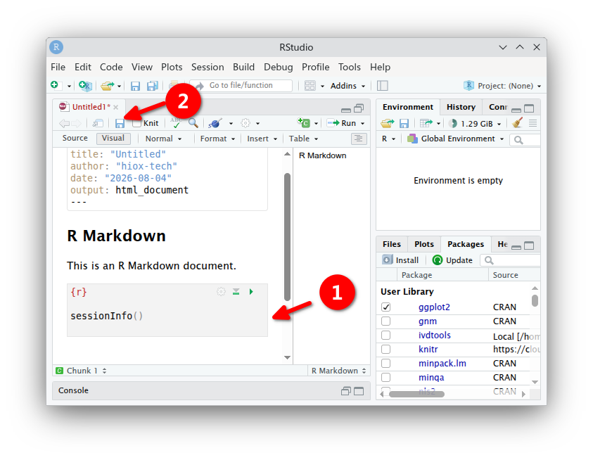

Recommended for archiving:

The unmodified raw data;
The .Rmd source file;
The rendered HTML/PDF;
Readable results and figures;
The sessionInfo() environment information;