17 Reference Intervals

This chapter introduces reference-interval establishment, method selection, and result reporting. A reference interval describes the distribution range of measurements in a target reference population. It is not a disease-diagnostic cutoff and does not automatically apply to populations with different age, sex, region, or measurement system; population definitions and inclusion/exclusion criteria must be reported with the statistical method.

Scope of Use

reference_interval() calculates a statistical interval for a defined sample set. It does not recruit reference individuals, determine partitions, justify sample size, investigate causes of outliers, or validate transfer across systems. Detection by an outlier test is not an automatic reason for exclusion, and a normality test does not replace a distribution plot. Reference coverage interval and endpoint confidence level ci are different parameters.

Workflow: establish and interpret a reference interval

%%{init: {"theme":"base","themeVariables":{"primaryColor":"#EAF2FB","primaryBorderColor":"#2780E3","primaryTextColor":"#212529","lineColor":"#6C757D","secondaryColor":"#EAF7E6","tertiaryColor":"#FFF4E8","fontSize":"13px"},"flowchart":{"nodeSpacing":18,"rankSpacing":24,"padding":6}}}%%

flowchart LR
    A["Define reference population<br/>and prespecified partitions"] --> B["outliers_test()<br/>normal_test()"]
    B --> C["reference_interval()"]
    C --> D["Prespecified primary method<br/>nonparametric or biweight"]
    C --> E["Sensitivity analyses<br/>type 6, parametric, Huber"]
    D --> F["Check endpoints and confidence intervals"]
    E --> F
    F --> G["Report separately from<br/>clinical decision limits"]

    classDef input fill:#EAF2FB,stroke:#2780E3,color:#212529
    classDef process fill:#EAF7E6,stroke:#3FB618,color:#212529
    classDef output fill:#F4EEFB,stroke:#9954BB,color:#212529
    class A input
    class B,C,D,E,F process
    class G output

A reference interval (RI) is defined by measurements in a reference sample population and is used to interpret individual results, corresponding to CLSI EP28-A3c. ivdtools uses the standard simple nonparametric method by default and implements the Appendix B biweight method. It also provides R type-6 quantiles with normal-approximation rank intervals, normal/log-normal parametric intervals, and Huber M robust intervals as explicitly named extensions. These methods differ in sensitivity to sample size, distribution shape, and outliers. Perform outlier and normality assessment before establishment; presenting multiple methods is a sensitivity comparison, not a post hoc choice of the most favorable result.

Code

library(ivdtools)
library(readr)

17.1 Main Functions

Function	Main purpose	Key inputs or outputs
`outliers_test()`	Outlier detection	Grubbs / ESD / Dixon / IQR
`normal_test()`	Normality test and plot	`method="auto"` selects by sample size
`reference_interval()`	Reference intervals by five methods	`method="all"`, `interval`, `ci`, bootstrap settings
`plot.reference_interval()`	Plot intervals by method	Jitter plus lower/upper limits

Code

reference_interval(
  data, col, interval = 0.95, ci = 0.95,
  method = "nonparametric",
  id = NULL,
  bootstrap_replicates = 1999,
  seed = NULL
)

Let the central coverage be \(γ\). The two-tail probability is

\[ \alpha=(1-γ)/2. \]

The five methods are defined as follows:

Method	Reference limits	Endpoint interval
`nonparametric` (default)	EP28 \(r=p(n+1)\) with linear interpolation at noninteger ranks	Order-statistic interval from binomial inversion, with actual coverage reported
`biweight`	EP28 Appendix B \(T_{bi}\), \(s_{bi}[205.6]\), and \(S_T[3.7]\)	Percentile bootstrap
`type6`	R `quantile(type=6)` at \(α\) and \(1-α\)	Retained normal-approximation rank positions
`parametric`	\(̅x±z_{1-α}s\)	t approximation for the SE of reference limits
`huber`	Huber location \(T±z_{1-α}S\)	Percentile bootstrap

The parametric method first performs Shapiro–Wilk. If normality is rejected and all values are positive, it tries a natural-log transformation; only if normality is not rejected after transformation does it calculate on the log scale and back-transform. If both original and log scales reject normality, the function warns and continues on the original scale. Biweight and Huber both start from the median and MAD, but use different weights, scales, and reference-limit formulas; they must not be treated as one generic “robust method.” bootstrap_replicates must be at least 100. Setting seed makes the bootstrap reproducible, and the function restores the caller’s random-number state.

Complete finite values in col enter the analysis; id is used only to report duplicate rows and does not automatically retain one row per person. The object stores nonparametric, biweight, type6, parametric, and huber results along with cleaned values. Showing all five methods is a sensitivity comparison, not a license to choose the most favorable method after seeing results.

outliers_test() and normal_test() return the method, statistic, P value, and indices. reference_interval() returns reference limits, endpoint confidence intervals, actual coverage, and cleaned data. plot.reference_interval() returns a ggplot object.

17.2 Analysis Examples

17.2.1 Example: Compare All Five Methods

This example performs prespecified outlier and normality checks and then calls reference_interval(method = "all") to output all five methods. The deterministic teaching data have \(n=120\), mild right skew, and outliers.

Code

ri_data <- read_csv("./data/017-参考区间/reference-interval.csv", show_col_types = FALSE)
ri_data <- as.data.frame(ri_data)

EP28 recommends reviewing outliers before establishing an RI. With \(n=120\), Dixon is not suitable (it is limited to \(n\le30\)), so use Grubbs and generalized ESD:

Code

outliers_test(ri_data, col = "value", method = "grubbs")

Grubbs Outliers Test
  Data:   ri_data
  Column: value (n = 120, missing = 0)
  Parameters: alpha = 0.05
  Outliers: 1

  Index            Value      G stat    Critical
  -------------------------------------------
  88            183.0000      4.0104      3.4451

Code

outliers_test(ri_data, col = "value", method = "esd", r = 3)

Generalized ESD Outliers Test
  Data:   ri_data
  Column: value (n = 120, missing = 0)
  Parameters: alpha = 0.05, r = 3
  Outliers: 2

  Index            Value      R stat    Critical
  -------------------------------------------
  88            183.0000      4.0104      3.4451
  57            178.0000      4.0576      3.4424

outliers_test() accepts "grubbs", "esd", "dixon", and "iqr"; ESD uses r for the maximum number of detections, Dixon uses type ("both", "min", or "max"), and IQR uses coef (default 1.5). Detecting an outlier does not mean it should be deleted. Review original records, the experimental process, and protocol, and perform inclusion/exclusion sensitivity analyses when justified.

Code

nt <- normal_test(ri_data, col = "value", method = "auto")
nt


Normality Test
  Data:   ri_data
  Column: value (n = 120, missing = 0)
  Method:     Anderson-Darling

  A = 1.7577, p = 0.0002

Code

plot(nt, type = c("qq", "his"))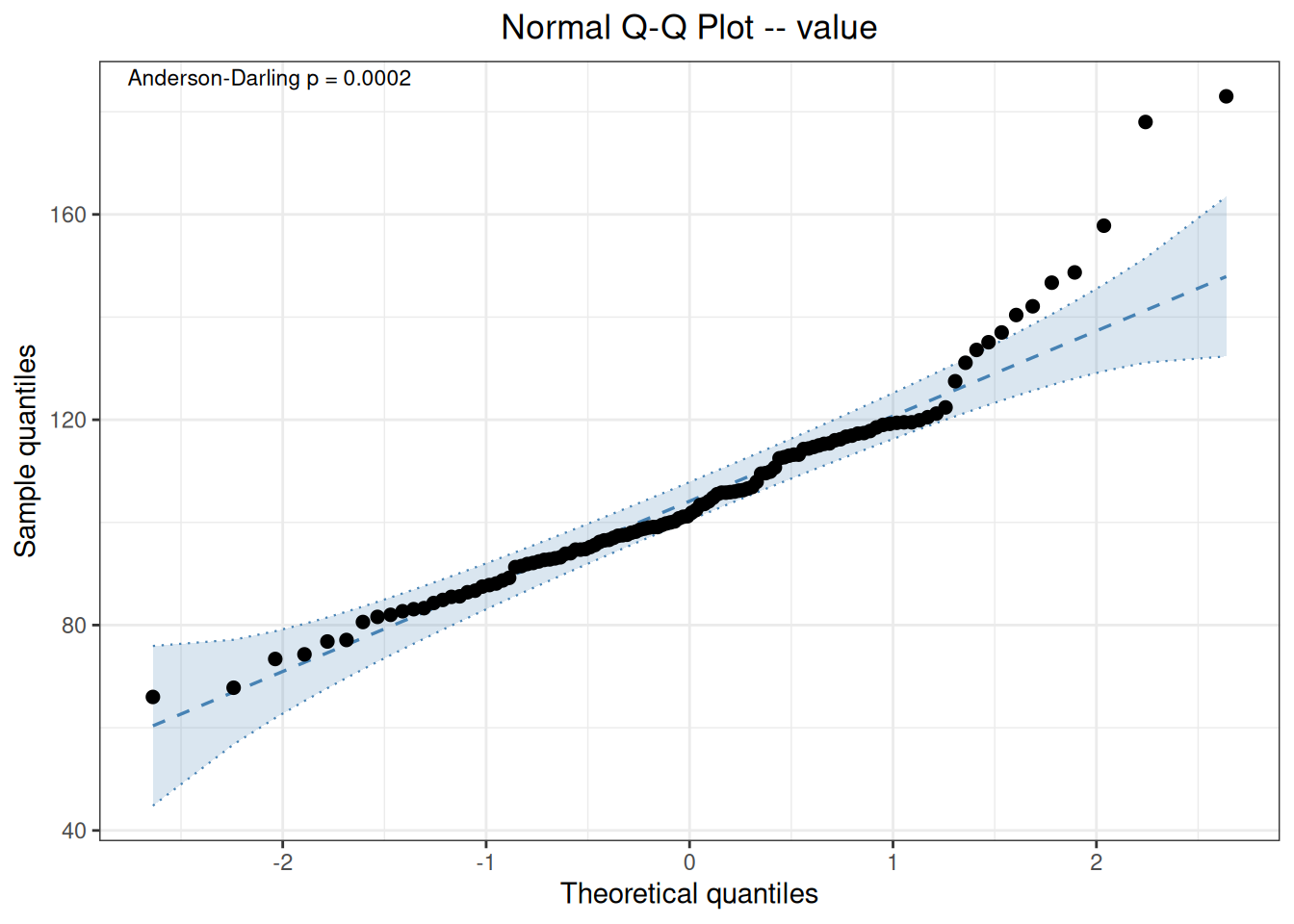

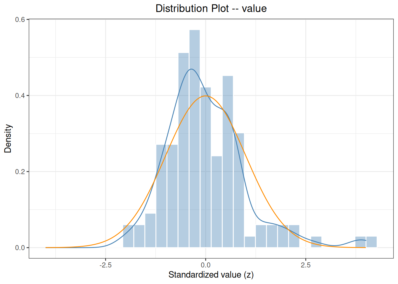
With \(n=120\), method="auto" selects the Anderson–Darling test. A small P value suggests non-normal data; the right-skewed distribution and outliers can be checked in the Q-Q plot and histogram.

Code

set.seed(1728)
ri <- reference_interval(
  ri_data,
  col = "value",
  interval = 0.95,
  ci = 0.95,
  method = "all",
  id = "id",
  bootstrap_replicates = 1999,
  seed = 1728
)
print(ri)


Reference Interval Analysis
  Column:              value
  Reference interval:  95% (alpha = 0.025)
  Confidence level:    0.95
  ID variable:         id
  Complete cases:      120 / 120

  No missing values.
  No duplicate IDs found.

  Nonparametric (CLSI EP28-A3c; exact binomial rank CI)
    Lower = 73.4225  [66.0000, 81.6000]
    Upper = 157.5725  [137.0000, 183.0000]
    Point ranks: 3.0250 and 117.9750
    CI ranks: lower 1-8; upper 113-120
    Actual rank coverage: lower 0.9412; upper 0.9412
    Warning: requested rank-CI coverage is not fully attainable at this sample size.

  Biweight (CLSI EP28-A3c Appendix B; 6 iterations)
    Lower = 63.2548  [54.4269, 71.4132]
    Upper = 141.7011  [133.3354, 149.8618]
    Tbi = 102.477938; sbi[205.6] = 19.748969; ST[3.7] = 1.536778
    Bootstrap valid: 1999 / 1999

  Type 6 (R quantile type 6; normal-approximation rank CI)
    Lower = 73.4225  [66.0000, 80.6000]
    Upper = 157.5725  [137.0000, 183.0000]

  Parametric (log-transformed, Shapiro-Wilk p = 0.0661)
    Lower = 73.2539  [69.3807, 77.3434]
    Upper = 145.9407  [138.2241, 154.0880]

  Huber (Huber M-estimation (k=1.5, 16 iter) + MAD)
    Lower = 72.1573  [66.8868, 77.1452]
    Upper = 134.7365  [128.8693, 142.7196]
    Bootstrap valid: 1999 / 1999

Code

plot(ri)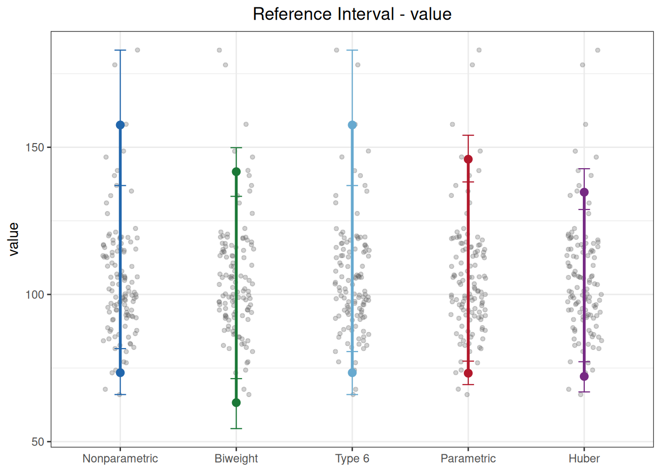

In reference_interval(), interval is reference-interval coverage (default 0.95, corresponding to 2.5%–97.5%) and ci is endpoint confidence level; they have different meanings. method can be any combination of "nonparametric", "biweight", "type6", "parametric", and "huber", or the single value "all". id is used for duplicate-sample detection.

The five methods in this example are:

Nonparametric (73.4–157.6): EP28 point estimates make no distributional assumption and endpoint CIs use binomial ranks.
Biweight (63.3–141.7): uses the two scale components from EP28 Appendix B; this teaching data set with outliers does not satisfy the prerequisite of investigating anomalies first.
Type 6 (73.4–157.6): point estimates match the nonparametric method, but endpoint CIs use retained normal-approximation ranks.
Parametric (73.3–145.9): after detecting non-normality, the function applies a log transformation (transformed=TRUE) and back-transforms.
Huber (72.2–134.7): based on Huber M estimation and MAD.

Differences among methods reflect different rank intervals, distributional assumptions, and robust-scale definitions.

17.2.2 Standard Case: CLSI EP28-A3c Appendix B Robust Iteration

Appendix B demonstrates the biweight calculation with 20 female calcium observations. This small sample is for algorithm demonstration only; the standard explicitly does not recommend it for establishing a formal RI. method="biweight" directly returns the location, scale components, reference limits, and bootstrap endpoint intervals from Appendix B.

Code

ep28_b <- as.data.frame(read_csv(
  "./data/017-参考区间/std-ep28-appendix-b.csv",
  show_col_types = FALSE
))
ep28_biweight <- reference_interval(
  ep28_b, col = "calcium", interval = 0.95,
  ci = 0.90, method = "biweight",
  bootstrap_replicates = 1999, seed = 2803
)
ep28_biweight


Reference Interval Analysis
  Column:              calcium
  Reference interval:  95% (alpha = 0.025)
  Confidence level:    0.9
  ID variable:         --
  Complete cases:      20 / 20

  No missing values.
  Note: 'id' not provided, skip duplicate detection.

  Biweight (CLSI EP28-A3c Appendix B; 6 iterations)
    Lower = 9.0495  [8.8339, 9.2781]
    Upper = 10.1994  [9.9725, 10.4052]
    Tbi = 9.624439; sbi[205.6] = 0.270427; ST[3.7] = 0.048187
    Bootstrap valid: 1989 / 1999

EP28 Appendix B: biweight intermediate values and reference limits
Standard position	Statistic	Standard result	ivdtools result
EP28-A3c Appendix B	Tbi	9.62440	9.62444
EP28-A3c Appendix B	sbi[205.6]	0.27043	0.27043
EP28-A3c Appendix B	ST[3.7]	0.04816	0.04819
EP28-A3c Appendix B	lower	9.05000	9.04951
EP28-A3c Appendix B	upper	10.20000	10.19937

The unrounded \(S_T\) differs from the displayed standard value by approximately \(2.7\times10^{-5}\), a rounding difference in an intermediate standard value, and is retained transparently in the table. A formal RI still requires a sample that meets the protocol; the standard explicitly states that 20 observations are for algorithm demonstration and that robust methods also require prior investigation of justified outliers.