3 Calibration Curve Fitting

This chapter demonstrates how to use fit_equation() from ivdtools to fit calibration curves and check convergence, residuals, the effect of weights, and forward and inverse predictions. The underlying implementation calls minpack.lm, nloptr, nls2, and stats.

Code

library(ivdtools)
library(readr)

3.1 Main Functions

Function	Purpose
`list_equation()`	View the built-in equation registry
`replicate_to_mean()`	Summarize replicate measurements and optionally calculate weights
`fit_equation()`	Fit a built-in or custom equation
`coef()`	Extract model parameters
`residuals()`	Extract observed-minus-fitted residuals
`predict()`	Predict response values forward or estimate concentrations inversely
`plot()`	Plot observed points, the fitted curve, and intervals
`compare_equation()`	Compare candidate equations

3.1.1 View Built-in Equations with `list_equation()`

Code

list_equation()

  ID       Name                         Formula        Params nP Engine
-----------------------------------------------------------------------
 E01     Linear                         a + b*x          a, b  2     lm
 E02  Quadratic                 a + b*x + c*x^2       a, b, c  3     lm
 E03 ExpoGrowth                  a * exp(b * x)          a, b  2    nls
 E04  ExpoDecay                 a * exp(-b * x)          a, b  2    nls
 E05      Power                         a * x^b          a, b  2    nls
 E06        Log                  a + b * log(x)          a, b  2     lm
 E07       4PLC   A + (B - A) / (1 + (x / C)^D)    A, B, C, D  4    nls
 E08       5PLC A + (B - A) / (1 + (x / C)^D)^E A, B, C, D, E  5    nls
 E09   Gaussian a * exp(-(x - b)^2 / (2 * c^2))       a, b, c  3    nls
 E10  Michaelis             Vmax * x / (Km + x)      Vmax, Km  2    nls
 E11 Sinusoidal          a * sin(b * x + c) + d    a, b, c, d  4    nls
 E12      Cubic         a + b*x + c*x^2 + d*x^3    a, b, c, d  4     lm

The function returns a registry data frame containing equation IDs, names, formulas, numbers of parameters, applicable categories, and fitting engines.

3.1.2 Summarize Replicates with `replicate_to_mean()`

If each concentration has replicate measurements, you can fit all observations directly or first summarize them with replicate_to_mean().

Code

replicate_to_mean(
  data, x = "Con", y = "RLU", weights = NULL, na.rm = TRUE
)

The function groups by x and returns summary fields such as the mean, number of replicates, and dispersion at each concentration. weights can provide numeric weights or a weighting rule for later fitting. na.rm = TRUE excludes missing rows; the number excluded should be recorded. Summary means are suitable for describing each level and should not automatically be treated as the error model for a future single specimen.

3.1.3 Fit a Built-in or Custom Equation with `fit_equation()`

fit_equation() accepts an ordinary data.frame. x is the concentration or relative concentration and y is the instrument response; both columns must contain finite numeric values.

fit_equation() can use automatic starting values or starting values supplied through start; lower, upper, and constraints can set parameter bounds or constraints. weights accepts a numeric vector or one of the built-in schemes "equal", "1/y", "1/y^2", "1/x", and "1/x^2".

Code

fit_equation(
  eq, data, x = "x", y = "y", start = NULL,
  lower = NULL, upper = NULL, constraints = NULL,
  weights = NULL, ...
)

The returned object has S3 class fit_equation and contains the selected equation, fitted model, parameters, data, and fitting diagnostics.

3.1.4 Compare Candidate Equations with `compare_equation()`

Main inputs

Code

compare_equation(
  data, x = "Con", y = "RLU", eqs = c("4PLC", "5PLC")
)

The returned object has S3 class compare_equation; its $table is sorted by AIC and includes at least Eq, Name, Formula, nPar, AIC, deltaAIC, R2, and RSE. AIC is evidence for comparing candidate models, not a replacement for residuals, plateau behavior, the reporting range, or external validation. If candidate models were not prespecified in the protocol, the comparison should be labeled exploratory.

3.1.5 Get Fitted Parameters and Residuals with `coef()` and `residuals()`

Code

coef(fit)
residuals(fit)

Here fit is the fitted object returned by fit_equation(). coef(fit) returns a named vector of fitted coefficients; residuals(fit) returns observed-minus-fitted residuals corresponding to valid observation rows.

3.1.6 Forward Response Prediction or Inverse Concentration Estimation with `predict()`

Code

predict(
  fit,
  newdata,
  interval = "confidence",
  level = 0.95,
  inverse = TRUE
)

newdata contains the concentrations or responses to predict. interval and level specify the interval type and confidence level. A confidence interval describes uncertainty in the fitted mean; a prediction interval also includes single-observation error and is usually wider. inverse requests inverse estimation of concentration from response.

The function returns a data frame containing input values, point predictions, and the requested lower and upper bounds. For inverse prediction, the point prediction is the estimated concentration.

Prediction Boundaries

Avoid extrapolating beyond the calibration concentration range. Inverse prediction is highly sensitive to response error on a plateau, and non-monotonic models may have multiple solutions.

3.1.7 Plot the Fitted Curve and Interval with `plot()`

Code

plot(fit, interval = "confidence", level = 0.95)

Use the figure to check observed points, the fitted curve, intervals, and the calibration range. A formal report should preserve the equation, weights, interval type, parameters, convergence status, and plotting parameters.

3.2 Analysis Examples

3.2.1 Fitting a Linear Calibration Curve

The linear equation is appropriate when the response changes with concentration at an approximately constant rate across the working range. In the ivdtools registry it corresponds to E01:

\[y = a + b x\]

Here $a$ is the intercept and $b$ is the slope. This example uses deterministic teaching data in data/003-校准曲线拟合/Linear.csv only to demonstrate the workflow. A formal calibration should define the concentration range, number of replicates, weights, and acceptance criteria in the study protocol.

Code

# Read the linear data file
fit_linear_data <- read_csv(
  "./data/003-校准曲线拟合/Linear.csv",
  show_col_types = FALSE
)

# Inspect the data structure
head(fit_linear_data, 6)

# A tibble: 6 × 3
  Sample   Con   RLU
  <chr>  <dbl> <dbl>
1 c1         0  1185
2 c2         5  3415
3 c3        10  5230
4 c4        20  9810
5 c5        40 18080
6 c6        60 26290

Code

# Fit the linear calibration curve
fit_linear <- fit_equation(
  "E01",
  data = fit_linear_data,
  x = "Con",
  y = "RLU"
)

# Display fitting results and parameters
print(fit_linear)

E01 (Linear)
Formula: a + b*x

Call:
  stats::lm(formula = frm, data = d, weights = weights)

Residuals:
      Min       1Q   Median       3Q      Max
    -736.970  -185.656  -38.780  151.657  693.530

Coefficients:
  Estimate Std. Error   t value   Pr(>|t|)    
a 1292.468  183.32973   7.04996 3.4988e-05 ***
b  418.525    1.87989 222.63236 < 2.22e-16 ***
---
Signif. codes:  0 '***' 0.001 '**' 0.01 '*' 0.05 '.' 0.1 ' ' 1

Residual standard error: 395.923 on 10 degrees of freedom
Multiple R-squared: 0.9998,  Adjusted R-squared: 0.9998
F-statistic: 49565.2 on 1 and 10 DF,  p-value: <2e-16

Code

coef(fit_linear)

       a        b 
1292.468  418.525

Code

# Plot observations, fitted line, and a 99% confidence interval for the mean
plot(fit_linear, interval = "confidence", level = 0.99)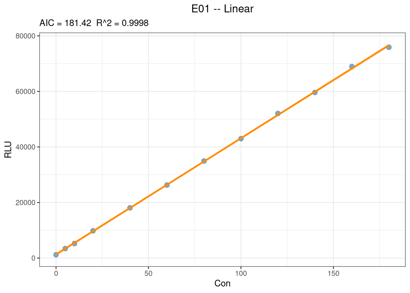

Code

# Predict response from concentration
predict(
  fit_linear,
  newdata = data.frame(Con = c(25, 75, 150)),
  interval = "confidence",
  level = 0.95
)

   x        y y_ci_lwr y_ci_upr
  25 11755.59 11422.52 12088.66
  75 32681.84 32427.13 32936.56
 150 64071.22 63670.87 64471.57

Code

# Estimate concentration inversely from response
predict(
  fit_linear,
  newdata = data.frame(RLU = c(10000, 30000, 60000)),
  inverse = TRUE
)

         x     y
  20.80529 10000
  68.59215 30000
 140.27246 60000

The slope represents the average rate at which response changes with concentration, and the intercept is the estimated response at concentration 0. Assess model suitability using residual trends, fitted intervals, back-calculated bias, and prespecified acceptance criteria; a high $R^2$ alone does not establish complete linearity across the calibration range. Inverse predictions should be restricted to the actual calibration range and should not be extrapolated without justification.

3.2.2 Fitting a 4PLC Calibration Curve for a Sandwich Assay

The four-parameter logistic (4PLC) model is nonlinear:

\[y = A + \frac{B-A}{1 + (x/C)^D}\]

Here $A$ and $B$ are the two asymptotic plateaus, $C$ is the concentration scale at the midpoint of the curve, and $D$ controls the direction and steepness. Interpret the parameters in light of the actual signal direction.

Code

# Read the data file
fit_4plc_data <- read_csv("./data/003-校准曲线拟合/4PLC.csv", show_col_types = FALSE)

# Inspect the data structure
head(fit_4plc_data, 6)

# A tibble: 6 × 3
  Sample   Con     RLU
  <chr>  <dbl>   <dbl>
1 c1      0       5637
2 c2      0.05   16014
3 c3      0.2    47520
4 c4      0.51  125038
5 c5      1.03  277621
6 c6      5.19 1498023

Code

# Fit the 4PLC curve with 1/y^2 weights
fit_4plc <- fit_equation(
  "4PLC",
  data = fit_4plc_data,
  x = "Con",
  y = "RLU",
  weights = "1/y^2"
)

# Display the fitting results
print(fit_4plc)

E07 (4PLC)
Formula: A + (B - A) / (1 + (x / C)^D)

Call:
  fit_equation(eq = "4PLC", data = fit_4plc_data, x = "Con", y = "RLU", 
      weights = "1/y^2")

Residuals:
      Min       1Q   Median       3Q      Max
    -1038926.254  -2031.562  491.283  35707.649  809345.965

Coefficients:
      Estimate  Std. Error    t value   Pr(>|t|)    
A  5.66828e+03 2.30614e+02   24.57907 4.7016e-08 ***
B  2.00185e+08 6.72603e+07    2.97627   0.020624 *  
C  4.83741e+02 1.74222e+02    2.77658   0.027433 *  
D -1.08082e+00 1.02400e-02 -105.54858 1.8062e-12 ***
---
Signif. codes:  0 '***' 0.001 '**' 0.01 '*' 0.05 '.' 0.1 ' ' 1

Residual standard error: 0.042025 on 7 degrees of freedom
AIC: 265.29  Iterations: 7

Code

# Obtain fitted residuals
residuals(fit_4plc)

 [1] -3.128012e+01  4.912832e+02 -2.231827e+03 -1.831297e+03  1.304427e+04
 [6]  1.466392e+04  5.675138e+04 -3.256634e+05  6.828909e+05 -1.038926e+06
[11]  8.093460e+05

Code

# Plot the curve
plot(fit_4plc, interval = "prediction", level = 0.95)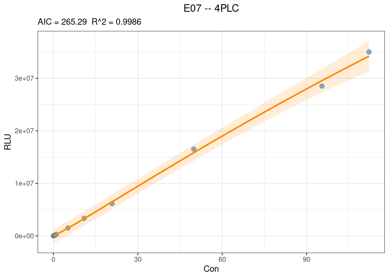

Code

# Predict y from x
predict(
  fit_4plc,
  newdata = data.frame(Con = c(20, 200, 1000)),
)

    x         y
   20   6205093
  200  55646993
 1000 137475699

Code

# Predict x from y
predict(
  fit_4plc,
  newdata = data.frame(RLU = c(10000, 100000, 1000000)),
  inverse = TRUE
)

        x     y
 0.023371 1e+04
 0.404396 1e+05
 3.589256 1e+06

3.2.3 Constrained Fitting

The following example reuses the linear data above and focuses on how to specify parameter constraints in fit_equation().

When theory says that the response should be 0 at concentration 0, or when the protocol explicitly requires that the intercept not be estimated, the intercept parameter $a$ can be fixed at 0:

Code

fit_linear_zero <- fit_equation(
  "E01",
  data = fit_linear_data,
  x = "Con",
  y = "RLU",
  constraints = list(eq = function(p) p["a"])
)

print(fit_linear_zero)

E01 (Linear)
Formula: a + b*x

Call:
  fit_equation(eq = "E01", data = fit_linear_data, x = "Con", y = "RLU", 
      constraints = list(eq = function(p) p["a"]))

Residuals:
      Min       1Q   Median       3Q      Max
    -1309.733  268.826  616.260  1002.094  1270.563

Coefficients:
                 Estimate Std. Error  t value Pr(>|t|)
  a              0.000000 447.987279    0.000 1       
  b            428.887404   4.594117   93.356 9.41e-15 ***
---
Signif. codes:  0 '***' 0.001 '**' 0.01 '*' 0.05 '.' 0.1 ' ' 1

Residual standard error: 1019.73 on 9 degrees of freedom
AIC: 166.80, R^2: 0.9988
Convergence: 4 (NLOPT_XTOL_REACHED: Optimization stopped because xtol_rel or xtol_abs (above) was reached.)

3.1 Main Functions

3.1.1 View Built-in Equations with list_equation()

3.1.2 Summarize Replicates with replicate_to_mean()

3.1.3 Fit a Built-in or Custom Equation with fit_equation()

3.1.4 Compare Candidate Equations with compare_equation()

3.1.5 Get Fitted Parameters and Residuals with coef() and residuals()

3.1.6 Forward Response Prediction or Inverse Concentration Estimation with predict()

3.1.7 Plot the Fitted Curve and Interval with plot()

3.2 Analysis Examples

3.2.1 Fitting a Linear Calibration Curve

3.2.2 Fitting a 4PLC Calibration Curve for a Sandwich Assay

3.2.3 Constrained Fitting

3.1.1 View Built-in Equations with `list_equation()`

3.1.2 Summarize Replicates with `replicate_to_mean()`

3.1.3 Fit a Built-in or Custom Equation with `fit_equation()`

3.1.4 Compare Candidate Equations with `compare_equation()`

3.1.5 Get Fitted Parameters and Residuals with `coef()` and `residuals()`

3.1.6 Forward Response Prediction or Inverse Concentration Estimation with `predict()`

3.1.7 Plot the Fitted Curve and Interval with `plot()`