15 Qualitative Analysis and C5/C95

This chapter addresses three different questions: whether binary results from a candidate and reference method agree, how strong the agreement between positive/negative classifications is, and where a continuous response reaches a specified detection probability near a critical concentration. The first two questions use paired four-fold tables; the last uses c5_c95().

Scope of Use

Before analysis, fix the positive direction, the reference method or clinical-state definition, the rule for combining replicate measurements, and the confidence-interval method. If a subject has multiple results, define a subject-level classification according to the protocol first; do not treat replicates as independent samples to inflate the sample size.

Workflow: from classification results to qualitative-performance conclusions

%%{init: {"theme":"base","themeVariables":{"primaryColor":"#EAF2FB","primaryBorderColor":"#2780E3","primaryTextColor":"#212529","lineColor":"#6C757D","secondaryColor":"#EAF7E6","tertiaryColor":"#FFF4E8","fontSize":"13px"},"flowchart":{"nodeSpacing":18,"rankSpacing":24,"padding":6}}}%%

flowchart LR
    A{"Input data level"} -->|case-level classifications| B["raw_to_table()"]
    A -->|TP/FP/TN/FN| C["counts_to_table()"]
    B --> D["diagnostics() / kappa()<br/>mcnemar()"]
    C --> D
    A -->|continuous internal response| E["continuous_to_binary()<br/>or c5_c95()"]
    D --> F["Clinical performance or<br/>observer agreement"]
    E --> G["Detection probability near threshold<br/>or claim verification"]

    classDef input fill:#EAF2FB,stroke:#2780E3,color:#212529
    classDef process fill:#EAF7E6,stroke:#3FB618,color:#212529
    classDef decision fill:#FFF4E8,stroke:#FF7518,color:#212529
    classDef output fill:#F4EEFB,stroke:#9954BB,color:#212529
    class A decision
    class B,C,D,E process
    class F,G output

Qualitative analysis evaluates agreement between candidate and reference positive/negative classifications, corresponding to CLSI EP12. ivdtools provides raw_to_table() to build a four-fold table from raw paired data, counts_to_table() to build one directly from TP/FP/TN/FN counts, and three analysis methods: diagnostics() (sensitivity, specificity, PPV, NPV, likelihood ratios, and so on), kappa() (Kappa and PABAK), and mcnemar() (paired-difference test). Use continuous_to_binary() when quantitative results must be converted to qualitative classifications.

Code

library(ivdtools)
library(readr)

15.1 Main Functions

Function	Main purpose	Key inputs or outputs
`raw_to_table()`	Build a four-fold table from raw paired data	`candidate`, `reference`, `positive`, `na.rm`
`counts_to_table()`	Build a four-fold table from TP/FP/TN/FN	`candidate`/`reference` labels
`continuous_to_binary()`	Convert quantitative results to qualitative classes	`cutoff` (≥ cutoff is 1)
`describe()`	Describe raw data	Available only for `raw_to_table()` sources
`diagnostics()`	Diagnostic accuracy metrics	`ci.method`, `prevalence`
`kappa()`	Kappa / PABAK	`prevalence` switch
`mcnemar()`	Paired-difference test	Exact test when discordant pairs <25
`c5_c95()`	C5/C95 from an internal continuous response	`cutoff`, `direction`, precision profile

Choose the function according to the data level. Use counts_to_table() when TP/FP/TN/FN are already available; use raw_to_table() for paired subject-level classifications; with only continuous signal and reference concentrations, first confirm that the replicate/precision relationship required by c5_c95() can be established. diagnostics(), kappa(), and mcnemar() all operate on the same four-fold table, so denominators must remain consistent in the report.

15.1.1 Four-Fold Metrics and Test Formulas

Code

raw_to_table(data, candidate, reference, id = NULL,
             na.rm = TRUE, positive = NULL)
counts_to_table(tp, fp, tn, fn,
                candidate = "candidate", reference = "reference")
diagnostics(object, conf.level = 0.95,
            ci.method = "wilson", prevalence = NULL)
kappa(x, prevalence = NULL, conf.level = 0.95)
mcnemar(x, conf.level = 0.95)

Let the four-fold table be \(a=TP,b=FP,c=FN,d=TN\). Main metrics are

\[ Se=\frac{a}{a+c},\quad Sp=\frac{d}{b+d},\quad PPV=\frac{a}{a+b},\quad NPV=\frac{d}{c+d}, \]

\[ LR^+=\frac{Se}{1-Sp},\qquad LR^-=\frac{1-Se}{Sp}. \]

diagnostics() can use Wilson, Wald, continuity-corrected Wald/Wilson, Agresti–Coull, Jeffreys, or Clopper–Pearson proportion intervals. When a target-population prevalence \(π\) is supplied, PPV/NPV are recalculated by Bayes’ theorem; the remaining metrics still come from the original table. When a cell is zero, log-approximation intervals for LR or OR may be NA; the function does not automatically apply a 0.5 correction.

Cohen’s Kappa is

\[ \kappa=\frac{P_o-P_e}{1-P_e},\qquad P_o=\frac{a+d}{n}, \]

where \(P_e\) is calculated from the marginal proportions of the two classifications. Passing prevalence to kappa() switches the current implementation to \(PABAK=2P_o-1\); this numeric argument triggers PABAK and records its label but does not enter the formula. McNemar uses only discordant pairs \(b,c\): when \(b+c<25\) it performs a two-sided exact binomial test; otherwise it uses the continuity-corrected statistic

\[ \chi^2=\frac{(|b-c|-1)^2}{b+c}. \]

raw_to_table() and counts_to_table() return four-fold-table objects; continuous_to_binary() returns a data frame with binary columns; describe() returns a descriptive table; and diagnostics(), kappa(), and mcnemar() return statistics, intervals, and test results.

15.1.2 C5/C95 Probability Model

Code

c5_c95(data, result = NULL, sample = NULL, cutoff,
       direction = c("geq", "leq"),
       probabilities = c(0.05, 0.95), component = NULL,
       model.no = 1:10, K = 2, search_range = NULL)

For an internal continuous-response mean \(μ\) and precision profile \(σ(μ)\), when direction="geq",

\[ P(\text{positive}\mid\mu) =1-\Phi\left(\frac{c-μ}{σ(μ)}\right). \]

C5/C95 are the values of \(μ\) at which this probability equals 0.05 and 0.95, respectively. Input may be raw replicate data or a precision object after variance() has been run. If there are multiple roots, the function selects the root closest to the cutoff; missing roots, multiple roots, and roots outside the observed-mean range are recorded in issues and should not be ignored.

c5_c95() returns C5/C95, the fitted model, and issues.

15.2 Analysis Examples

15.2.1 Example 1: Complete Analysis of Raw Paired Data

Code

qual <- read_csv("./data/015-定性分析与C5C95/qualitative-raw.csv", show_col_types = FALSE)
qual <- as.data.frame(qual)

qa <- raw_to_table(
  qual,
  candidate = "new",
  reference = "gold",
  id = "id",
  positive = "positive"
)
qa


Fourfold Table
  Source            : raw data
  Total n           : 60
  Duplicate IDs     : none
  Candidate         : new
  Reference         : gold

  2x2 Contingency Table
  ---------------------------------------- 
              gold                       
                  positive  negative  Sum       
  ---------------------------------------- 
  new   positive  23        1         24        
        negative  1         35        36        
        sum       24        36        60        
  ----------------------------------------

raw_to_table() requires exactly two levels in both candidate and reference columns; positive specifies the positive level for factor/character mapping; na.rm controls whether missing rows are removed. id is optional and is used to detect duplicate samples.

Code

qa <- describe(qa)


Data Summary
  Rows:    60
  Columns: 5
  ID:      60 unique, no duplicates

  new
    negative        36  ( 60.0%)
    positive        24  ( 40.0%)
  gold
    negative        36  ( 60.0%)
    positive        24  ( 40.0%)
  age
    Mean (SD):       51.05 (13.45)
    Median (Q1-Q3):  48.90 (42.15 - 57.28)
    Range:           24.30 - 90.10
  gender
    F               32  ( 53.3%)
    M               28  ( 46.7%)

describe() is available only for raw_to_table() sources and reports row count, duplicate IDs, column summaries, and missingness.

Code

qa <- diagnostics(qa, ci.method = "wilson")


Diagnostic Performance Summary
  Sensitivity        0.958  (0.798, 0.993) 
  Specificity        0.972  (0.858, 0.995) 
  PPV                0.958  (0.798, 0.993) 
  NPV                0.972  (0.858, 0.995) 
  Accuracy           0.967  (0.886, 0.991) 
  Prevalence         0.400  (0.286, 0.526) 
  LR+                34.500  (4.986, 238.724) 
  LR-                0.043  (0.006, 0.292) 
  Odds Ratio         805.000  (47.921, 13522.837) 

  # PPV & NPV are based on data prevalence of 0.400.
  # Confidence intervals for proportions use 'wilson' method.

Sensitivity is 0.958 and specificity is 0.972 in this example. If target-population prevalence is known, use prevalence to recalculate PPV/NPV:

Code

qa <- diagnostics(qa, prevalence = 0.4)


Diagnostic Performance Summary
  Sensitivity        0.958  (0.798, 0.993) 
  Specificity        0.972  (0.858, 0.995) 
  PPV                0.958  (0.790, 0.993) 
  NPV                0.972  (0.864, 0.995) 
  Accuracy           0.967  (0.886, 0.991) 
  Prevalence         0.400 
  LR+                34.500  (4.986, 238.724) 
  LR-                0.043  (0.006, 0.292) 
  Odds Ratio         805.000  (47.921, 13522.837) 

  # PPV & NPV are based on user-specified prevalence of 0.400.
  # Confidence intervals for proportions use 'wilson' method.

diagnostics() supports seven proportion confidence-interval methods (default "wilson"). With prevalence, PPV/NPV use Bayes’ theorem; otherwise they use the observed prevalence.

Code

qa <- kappa(qa)


Cohen's Kappa
  new  vs  gold
  n = 60

  Kappa                 0.9306
  SE                    0.0483
  95% CI                (0.8359, 1.0000)
  Observed agreement    0.9667
  Expected agreement    0.5200

Code

qa <- kappa(qa, prevalence = 0.5)


PABAK
  new  vs  gold
  n = 60

  Kappa                 0.9333
  SE                    0.0463
  95% CI                (0.8425, 1.0000)
  Observed agreement    0.9667
  Expected agreement    0.5000
  # PABAK (prevalence = 0.500): 2 * p_obs - 1, assumes expected agreement = 0.5

kappa() returns Cohen’s Kappa; with prevalence it instead computes PABAK (2·p_obs − 1). These handle prevalence bias differently, so report the method.

Code

qa <- mcnemar(qa)


McNemar Test
  new  vs  gold
  Discordant pairs:  b (pos, neg) = 1,  c (neg, pos) = 1
  n (b + c)        = 2

  Method: Exact binomial test
  P-value:          1.0000
  Conclusion: Not significant at 95% confidence level

Discordant pairs satisfy \(b+c=2<25\), so the function automatically uses the exact binomial test.

Code

summary(qa)


Qualitative Analysis - summary
-------------------------------------------------

Fourfold Table
  Source            : raw data
  Total n           : 60
  Duplicate IDs     : none
  Candidate         : new
  Reference         : gold

  2x2 Contingency Table
  ---------------------------------------- 
              gold                       
                  positive  negative  Sum       
  ---------------------------------------- 
  new   positive  23        1         24        
        negative  1         35        36        
        sum       24        36        60        
  ---------------------------------------- 

Analyses performed:

  [x] Describe
  [x] Diagnostics
  [x] Kappa
  [x] McNemar

Data Summary
  Rows:    60
  Columns: 5
  ID:      60 unique, no duplicates

  new
    negative        36  ( 60.0%)
    positive        24  ( 40.0%)
  gold
    negative        36  ( 60.0%)
    positive        24  ( 40.0%)
  age
    Mean (SD):       51.05 (13.45)
    Median (Q1-Q3):  48.90 (42.15 - 57.28)
    Range:           24.30 - 90.10
  gender
    F               32  ( 53.3%)
    M               28  ( 46.7%)

Diagnostic Performance Summary
  Sensitivity        0.958  (0.798, 0.993) 
  Specificity        0.972  (0.858, 0.995) 
  PPV                0.958  (0.790, 0.993) 
  NPV                0.972  (0.864, 0.995) 
  Accuracy           0.967  (0.886, 0.991) 
  Prevalence         0.400 
  LR+                34.500  (4.986, 238.724) 
  LR-                0.043  (0.006, 0.292) 
  Odds Ratio         805.000  (47.921, 13522.837) 

  # PPV & NPV are based on user-specified prevalence of 0.400.
  # Confidence intervals for proportions use 'wilson' method.

PABAK
  new  vs  gold
  n = 60

  Kappa                 0.9333
  SE                    0.0463
  95% CI                (0.8425, 1.0000)
  Observed agreement    0.9667
  Expected agreement    0.5000
  # PABAK (prevalence = 0.500): 2 * p_obs - 1, assumes expected agreement = 0.5

McNemar Test
  new  vs  gold
  Discordant pairs:  b (pos, neg) = 1,  c (neg, pos) = 1
  n (b + c)        = 2

  Method: Exact binomial test
  P-value:          1.0000
  Conclusion: Not significant at 95% confidence level

15.2.2 Example 2: Build Directly from TP/FP/TN/FN

When counts are already available, raw data are not needed:

Code

tab <- counts_to_table(
  tp = 80, fp = 5, tn = 120, fn = 3,
  candidate = "new method",
  reference = "gold standard"
)
tab


Fourfold Table
  Source            : counts
  Total n           : 208
  Candidate         : new method
  Reference         : gold standard

  2x2 Contingency Table
  ----------------------------------------------- 
                     gold standard              
                         positive  negative  Sum       
  ----------------------------------------------- 
  new method   positive  80        5         85        
               negative  3         120       123       
               sum       83        125       208       
  -----------------------------------------------

Code

tab <- diagnostics(tab)


Diagnostic Performance Summary
  Sensitivity        0.964  (0.899, 0.988) 
  Specificity        0.960  (0.910, 0.983) 
  PPV                0.941  (0.870, 0.975) 
  NPV                0.976  (0.931, 0.992) 
  Accuracy           0.962  (0.926, 0.980) 
  Prevalence         0.399  (0.335, 0.467) 
  LR+                24.096  (10.198, 56.934) 
  LR-                0.038  (0.012, 0.114) 
  Odds Ratio         640.000  (148.773, 2753.180) 

  # PPV & NPV are based on data prevalence of 0.399.
  # Confidence intervals for proportions use 'wilson' method.

Code

tab <- kappa(tab)


Cohen's Kappa
  new method  vs  gold standard
  n = 208

  Kappa                 0.9201
  SE                    0.0277
  95% CI                (0.8659, 0.9744)
  Observed agreement    0.9615
  Expected agreement    0.5184

Code

tab <- mcnemar(tab)


McNemar Test
  new method  vs  gold standard
  Discordant pairs:  b (pos, neg) = 5,  c (neg, pos) = 3
  n (b + c)        = 8

  Method: Exact binomial test
  P-value:          0.7266
  Conclusion: Not significant at 95% confidence level

Code

describe(tab)   # count sources have no raw data; describe() is unavailable

Objects built by counts_to_table() have no raw data, so describe() is unavailable; diagnostics(), kappa(), and mcnemar() work normally.

15.2.3 Example 3: Convert Quantitative Data to Qualitative

The candidate method is the quantitative result result and the reference is the qualitative variable gold:

Code

cont <- read_csv("./data/015-定性分析与C5C95/qualitative-continuous.csv", show_col_types = FALSE)
cont <- as.data.frame(cont)
head(cont, 6)

    id    result     gold
1 S001 10.111087 positive
2 S002 13.057209 positive
3 S003  1.534680 negative
4 S004  7.782787 negative
5 S005  4.982424 negative
6 S006  9.443399 negative

Convert to binary at cutoff 8:

Code

cont_bin <- continuous_to_binary(cont, cols = "result", cutoff = 8)
head(cont_bin, 6)

    id    result     gold result_binary
1 S001 10.111087 positive             1
2 S002 13.057209 positive             1
3 S003  1.534680 negative             0
4 S004  7.782787 negative             0
5 S005  4.982424 negative             0
6 S006  9.443399 negative             1

continuous_to_binary() creates result_binary (>= cutoff is 1, otherwise 0). To satisfy the positive mapping requirement of raw_to_table(), relabel it consistently with the reference:

Code

cont_bin$result_binary_lab <- ifelse(cont_bin$result_binary == 1, "positive", "negative")

Code

qa3 <- raw_to_table(
  cont_bin,
  candidate = "result_binary_lab",
  reference = "gold",
  id = "id",
  positive = "positive"
)
qa3 <- diagnostics(qa3)


Diagnostic Performance Summary
  Sensitivity        0.952  (0.773, 0.992) 
  Specificity        0.897  (0.736, 0.964) 
  PPV                0.870  (0.679, 0.955) 
  NPV                0.963  (0.817, 0.993) 
  Accuracy           0.920  (0.812, 0.968) 
  Prevalence         0.420  (0.294, 0.558) 
  LR+                9.206  (3.140, 26.994) 
  LR-                0.053  (0.008, 0.361) 
  Odds Ratio         173.333  (16.746, 1794.100) 

  # PPV & NPV are based on data prevalence of 0.420.
  # Confidence intervals for proportions use 'wilson' method.

The level supplied to positive must exist in both columns, so relabel the binary column as positive/negative first. If positive is omitted, the function may reverse the positive/negative direction according to sorted levels and flip TP/FP; always check.

15.2.4 Example 4: Estimate C5/C95 from an Internal Continuous Response

When a qualitative classification is based on an internal continuous signal and a fixed cutoff, use replicate measurements to establish an SD–mean precision profile and then find the mean response at the specified positive probabilities. Here result >= 40 defines the target event:

Code

head(c5_data, 6)

  level response
1    L1 35.14000
2    L1 35.29636
3    L1 35.45273
4    L1 35.60909
5    L1 35.76545
6    L1 35.92182

Code

c5_result <- c5_c95(
  c5_data,
  result = "response",
  sample = "level",
  cutoff = 40,
  direction = "geq",
  probabilities = c(0.05, 0.95),
  model.no = 1
)
c5_result

C5/C95 estimation from an internal continuous response
  Source: raw data
  Precision component: repeatability
  Event: response >= cutoff
 cutoff label probability mean_response     SD actual_probability extrapolated
------------------------------------------------------------------------------
     40    C5        0.05       39.0291 0.5903               0.05        FALSE
     40   C95        0.95       40.9709 0.5903               0.95        FALSE

Code

plot(c5_result, type = "probability")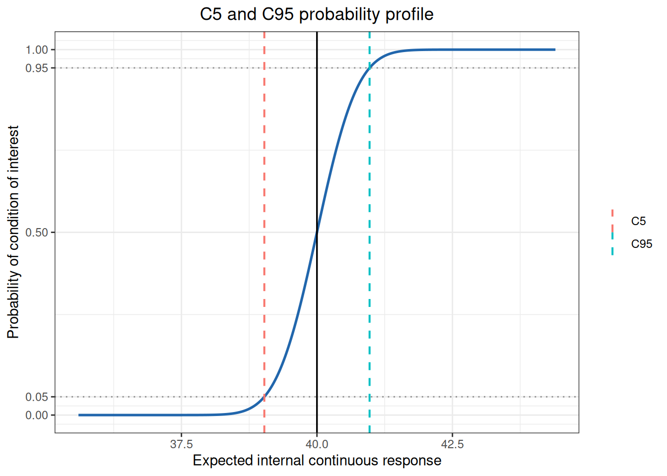

direction = "geq" means a response greater than or equal to the cutoff is the target event; "leq" means less than or equal to the cutoff. If a root lies outside the observed mean range, the object marks extrapolation. The precision-profile model and its coverage range should be included in the interpretation.