7 Interference Studies

Interference studies ask whether a potential interferent changes a measurement, how the effect changes with interferent concentration, and whether patient samples containing the factor show a larger method difference or dispersion. These are different analysis paths and should not be collapsed into one summary number.

Path	Main question	Main result
Paired preparation screen	Is the test sample sufficiently different from the solvent control at specified analyte/interferent levels?	Absolute/relative effect and confidence interval
Dose response	How does the effect change with interferent concentration?	Baseline-relative effect, monotonicity, interpolation
Patient-sample comparison	Do patient samples with the factor show method differences or increased dispersion?	Per-sample difference, group summary, difference–interferent regression

Scope of Use

Interference conclusions require prespecified interferents, concentrations, replicates, direction, and allowable effect. A statistical difference is not automatically clinically or analytically important. Keep the preparation design, solvent control, patient grouping, and method-difference direction explicit.

Code

library(ivdtools)
library(readr)

7.1 Main Functions

Function	Purpose	Return value
`interference_replicates()`	Calculate required test and control replicates	`interference_replicates` data frame
`interference_paired()`	Analyze paired-preparation interference	`interference_paired` object
`interference_dose_response()`	Analyze interferent dose response	`interference_dose_response` object
`predict()`	Forward or inverse prediction from a dose-response result	Prediction data frame
`interference_patient()`	Analyze method differences in patient samples	`interference_patient` object

7.1.1 Replicate Planning

Code

interference_replicates(
  sd, detectable_difference, alpha = 0.05, power = 0.90,
  alternative = c("two.sided", "one.sided"), min_replicates = 5,
  label = NULL
)

sd is expected repeatability SD, or repeatability CV on a relative scale. detectable_difference uses the same scale and compatible length. alpha and power must be finite values between 0 and 1; alternative determines one- or two-sided planning. The result is a design quantity, not an acceptance decision.

7.1.2 Paired-Preparation Studies

Code

interference_paired(
  data, result, design = c("ep07", "analyte_spike", "blank"),
  by = NULL, condition = NULL, test_level = NULL, control_level = NULL,
  matrix = NULL, normal_level = NULL, interferent_level = NULL,
  spike = NULL, unspiked_level = NULL, spiked_level = NULL,
  conf.level = 0.95
)

The data are long format, one replicate per row. For ep07, identify test and solvent-control conditions; for analyte_spike, identify normal/interferent matrix and unspiked/spiked analyte; for blank, identify the relevant condition. The returned object contains paired effects, relative effects, standard errors, intervals, and group summaries.

7.1.3 Dose–Response Studies

Code

interference_dose_response(
  data, result, concentration, by = NULL, baseline,
  method = c("point_to_point", "linear"), conf.level = 0.95
)

baseline must be an observed interferent concentration in every stratum. point_to_point interpolates adjacent concentration means; linear fits a straight line to individual results. The object preserves the baseline-relative effect, model coefficients, and predictions.

7.1.4 Patient-Sample Comparison

Code

interference_patient(
  data, id, group, method, result,
  test_group, control_group, evaluated_method, comparative_method,
  interferent_cols = NULL, conf.level = 0.95
)

The difference is defined as evaluated method minus comparative method. Optional interferent columns are fitted one at a time; group summaries and regression intervals use the specified confidence level.

7.2 Analysis Examples

7.2.1 EP07 Replicate Planning and Paired Screening

Code

ep07_paired <- as.data.frame(read_csv(
  "./data/007-干扰研究/std-ep07-table3-paired.csv",
  show_col_types = FALSE
))
ep07_fit <- interference_paired(
  ep07_paired, result = "result", design = "ep07",
  by = "level", condition = "condition",
  test_level = "test", control_level = "control", conf.level = 0.95
)
print(ep07_fit)

Interference paired-difference analysis
  Design: ep07
  Confidence level: 95%
  level: low
    stratum             : level=low
    design              : ep07
    n_test              : 5
    n_control           : 5
    test_mean           : 0.3
    control_mean        : 0.5
    absolute_difference : -0.2
    absolute_se         : 0.033166248
    df                  : 8
    absolute_ci_lower   : -0.2764815
    absolute_ci_upper   : -0.1235185
    percent_difference  : -40
    percent_se          : 6.6332496
    percent_ci_lower    : -55.296301
    percent_ci_upper    : -24.703699

  level: high
    stratum             : level=high
    design              : ep07
    n_test              : 5
    n_control           : 5
    test_mean           : 4.55
    control_mean        : 5
    absolute_difference : -0.45
    absolute_se         : 0.096436508
    df                  : 8
    absolute_ci_lower   : -0.67238299
    absolute_ci_upper   : -0.22761701
    percent_difference  : -9
    percent_se          : 1.9287302
    percent_ci_lower    : -13.44766
    percent_ci_upper    : -4.5523403

7.2.2 EP07 Dose Response

Code

ep07_dose <- as.data.frame(read_csv(
  "./data/007-干扰研究/std-ep07-table4-dose-response.csv",
  show_col_types = FALSE
))
ep07_dose_fit <- interference_dose_response(
  ep07_dose, result = "result", concentration = "concentration",
  baseline = 0, method = "point_to_point"
)
print(ep07_dose_fit)

Interference dose-response analysis
  Method: point_to_point
  Baseline concentration: 0
  Stratum: all | Concentration: 0
    Observations        : 5
    Mean                : 200.02
    SD                  : 1.7753873
    SE                  : 0.79397733
    Absolute difference : 0
    Percent difference  : 0
    CV percent          : 0.88760488

  Stratum: all | Concentration: 10
    Observations        : 5
    Mean                : 223.9
    SD                  : 4.645966
    SE                  : 2.0777392
    Absolute difference : 23.88
    Percent difference  : 11.938806
    CV percent          : 2.0750183

  Stratum: all | Concentration: 20
    Observations        : 5
    Mean                : 240.08
    SD                  : 3.3536547
    SE                  : 1.4998
    Absolute difference : 40.06
    Percent difference  : 20.027997
    CV percent          : 1.3968905

  Stratum: all | Concentration: 30
    Observations        : 5
    Mean                : 245.72
    SD                  : 4.7892588
    SE                  : 2.1418217
    Absolute difference : 45.7
    Percent difference  : 22.847715
    CV percent          : 1.9490716

  Stratum: all | Concentration: 40
    Observations        : 5
    Mean                : 251.88
    SD                  : 4.4549972
    SE                  : 1.9923353
    Absolute difference : 51.86
    Percent difference  : 25.927407
    CV percent          : 1.7686983

Code

plot(ep07_dose_fit)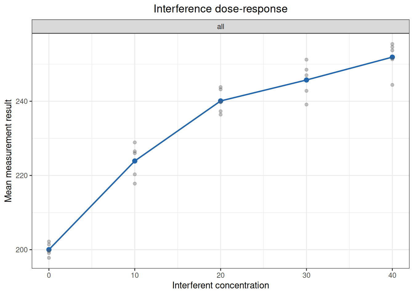

7.2.3 Patient-Sample Comparison

Code

patient_data <- as.data.frame(read_csv(
  "./data/007-干扰研究/std-yyt1789-5-appendix-c-patient.csv",
  show_col_types = FALSE
))
patient_fit <- interference_patient(
  patient_data, id = "id", group = "group", method = "method",
  result = "result", test_group = "test", control_group = "control",
  evaluated_method = "evaluated", comparative_method = "comparative"
)
print(patient_fit)

Patient-specimen interference evaluation
  Evaluated - comparative: evaluated - comparative
  Group: test
    Observations            : 20
    Mean difference         : -1.1835
    SD difference           : 2.3930541
    SE difference           : 0.53510317
    Median difference       : -0.49
    25th percentile         : -1.3425
    75th percentile         : -0.32
    CI lower                : -2.3034838
    CI upper                : -0.063516183
    Mean percent difference : -17.916419
    SD percent difference   : 18.774944
    Percent CI lower        : -26.703363
    Percent CI upper        : -9.1294749

  Group: control
    Observations            : 20
    Mean difference         : -1.039
    SD difference           : 2.1614978
    SE difference           : 0.4833256
    Median difference       : -0.415
    25th percentile         : -0.835
    75th percentile         : -0.075
    CI lower                : -2.0506121
    CI upper                : -0.027387902
    Mean percent difference : -11.712959
    SD percent difference   : 24.21947
    Percent CI lower        : -23.04802
    Percent CI upper        : -0.37789805

7.3 Interpretation and Reporting

Report the design, interferent and concentration, control preparation, replicate count, effect definition, confidence method, and allowable effect. A dose-response line can describe an association without proving mechanism. A patient-sample regression can be confounded by disease severity, sample matrix, or method range. EP07 and YY/T 1789.5 standard examples in the supplied data directory can be cross-checked with the same functions, but standard-specific acceptance limits and study conclusions remain external to the package.

7.4 Full Standard Cases

7.4.1 CLSI EP07 Third Edition Section 5.1: Replicate-Count Design

Section 5.1.1 of EP07 uses a two-sided example with repeatability SD 1.0 mg/dL, 95% confidence, 95% power, and a detectable effect of 1.5 mg/dL. Section 5.1.4 assumes a repeatability CV of 5% and detects effects of 7% and 10% with 95% confidence and 90% power. SD and difference, or CV and percentage difference, are on matching scales, so the same formula can be used.

Code

ep07_replicates_511 <- interference_replicates(
  sd = 1,
  detectable_difference = 1.5,
  alpha = 0.05,
  power = 0.95,
  label = "5.1.1 two-sided"
)
ep07_replicates_514 <- interference_replicates(
  sd = c(5, 5),
  detectable_difference = c(7, 10),
  alpha = 0.05,
  power = 0.90,
  label = c("5.1.4 7%", "5.1.4 10%")
)
rbind(ep07_replicates_511, ep07_replicates_514)

EP07 paired-difference replicate design
  Label: 5.1.1 two-sided
    SD                    : 1
    Detectable difference : 1.5
    Difference / SD       : 1.5
    Alpha                 : 0.05
    Power                 : 0.95
    Alternative           : two.sided
    Z alpha               : 1.959964
    Z power               : 1.6448536
    Calculated replicates : 11.550853
    Replicates per sample : 12
    Minimum replicates    : 5

  Label: 5.1.4 7%
    SD                    : 5
    Detectable difference : 7
    Difference / SD       : 1.4
    Alpha                 : 0.05
    Power                 : 0.9
    Alternative           : two.sided
    Z alpha               : 1.959964
    Z power               : 1.2815516
    Calculated replicates : 10.72186
    Replicates per sample : 11
    Minimum replicates    : 5

  Label: 5.1.4 10%
    SD                    : 5
    Detectable difference : 10
    Difference / SD       : 2
    Alpha                 : 0.05
    Power                 : 0.9
    Alternative           : two.sided
    Z alpha               : 1.959964
    Z power               : 1.2815516
    Calculated replicates : 5.2537115
    Replicates per sample : 6
    Minimum replicates    : 5

EP07 Section 5.1: replicate-count comparison
Standard position	Standard calculated	ivdtools calculated	Standard replicates	ivdtools replicates
5.1.1 two-sided	11.550853	11.550853	12	12
5.1.4 7%	10.721860	10.721860	11	11
5.1.4 10%	5.253712	5.253712	6	6

The replicate count must be satisfied separately for every test sample and control sample; the two groups must not be added together and interpreted as one total sample size.

7.4.2 CLSI EP07 Third Edition Table 3: Paired Screening

EP07 Table 3 compares five test replicates with five solvent-control replicates at analyte levels 0.50 and 5.00 mg/dL and an interferent concentration of 500 mg/dL. The effect direction is consistently test − control; use the absolute difference at the low level and the percentage difference relative to the control mean at the high level.

Code

ep07_table3 <- read_csv(
  "./data/007-干扰研究/std-ep07-table3-paired.csv",
  show_col_types = FALSE
)
head(ep07_table3, 6)

# A tibble: 6 × 5
  level condition replicate result unit 
  <chr> <chr>         <dbl>  <dbl> <chr>
1 low   control           1   0.45 mg/dL
2 low   control           2   0.56 mg/dL
3 low   control           3   0.48 mg/dL
4 low   control           4   0.54 mg/dL
5 low   control           5   0.47 mg/dL
6 low   test              1   0.24 mg/dL

Code

ep07_table3_result <- interference_paired(
  as.data.frame(ep07_table3),
  result = "result",
  design = "ep07",
  condition = "condition",
  test_level = "test",
  control_level = "control",
  by = "level",
  conf.level = 0.95
)
ep07_table3_result

Interference paired-difference analysis
  Design: ep07
  Confidence level: 95%
  level: low
    stratum             : level=low
    design              : ep07
    n_test              : 5
    n_control           : 5
    test_mean           : 0.3
    control_mean        : 0.5
    absolute_difference : -0.2
    absolute_se         : 0.033166248
    df                  : 8
    absolute_ci_lower   : -0.2764815
    absolute_ci_upper   : -0.1235185
    percent_difference  : -40
    percent_se          : 6.6332496
    percent_ci_lower    : -55.296301
    percent_ci_upper    : -24.703699

  level: high
    stratum             : level=high
    design              : ep07
    n_test              : 5
    n_control           : 5
    test_mean           : 4.55
    control_mean        : 5
    absolute_difference : -0.45
    absolute_se         : 0.096436508
    df                  : 8
    absolute_ci_lower   : -0.67238299
    absolute_ci_upper   : -0.22761701
    percent_difference  : -9
    percent_se          : 1.9287302
    percent_ci_lower    : -13.44766
    percent_ci_upper    : -4.5523403

The recalculated low-level control/test means are 0.50/0.30 mg/dL, with an absolute effect of −0.20 mg/dL and a 95% CI of −0.28 to −0.12 mg/dL. The high-level means are 5.00/4.55 mg/dL, with a relative effect of −9.0% and a 95% CI of −13.4% to −4.6% in ascending order. The standard prints the high-level interval in reverse order; only the display order is changed here.

EP07 Third Edition Table 3: comparison of ivdtools and standard results
level	statistic	standard	ivdtools
low	control_mean	0.500	0.5000
low	test_mean	0.300	0.3000
low	control_sd	0.047	0.0474
low	test_sd	0.057	0.0570
low	difference	-0.200	-0.2000
low	ci_lower	-0.280	-0.2765
low	ci_upper	-0.120	-0.1235
high	control_mean	5.000	5.0000
high	test_mean	4.550	4.5500
high	control_sd	0.141	0.1409
high	test_sd	0.163	0.1632
high	difference_percent	-9.000	-9.0000
high	ci_lower_percent	-13.400	-13.4477
high	ci_upper_percent	-4.600	-4.5523

Under the case’s prespecified limits, the low-level point estimate of −0.20 mg/dL exceeds ±0.10 mg/dL, while the high-level point estimate of −9.0% is within ±10%; this screening case therefore reports interference only at the low level. If equivalence is prespecified, the entire confidence interval should instead be required to lie within the allowable difference.

7.4.3 CLSI EP07 Third Edition Table 4: Curved Dose–Response and Point-to-Point Interpolation

EP07 Table 4 presents simulated dose–response data: interferent concentrations of 0, 10, 20, 30, and 40 mg/dL, with five measurements at each concentration. The analyte results are expressed in nmol/L. The means increase monotonically with interferent concentration but gradually flatten at high concentrations, so the main text uses a point-to-point method between adjacent means rather than summarizing the full range with one straight line.

Code

ep07_table4 <- read_csv(
  "./data/007-干扰研究/std-ep07-table4-dose-response.csv",
  show_col_types = FALSE
)
head(ep07_table4, 6)

# A tibble: 6 × 6
  sample replicate concentration result concentration_unit result_unit
   <dbl>     <dbl>         <dbl>  <dbl> <chr>              <chr>      
1      1         1             0   201. mg/dL              nmol/L     
2      1         2             0   199. mg/dL              nmol/L     
3      1         3             0   198. mg/dL              nmol/L     
4      1         4             0   200. mg/dL              nmol/L     
5      1         5             0   202. mg/dL              nmol/L     
6      2         1            10   218. mg/dL              nmol/L

Code

ep07_table4_result <- interference_dose_response(
  ep07_table4,
  result = "result",
  concentration = "concentration",
  baseline = 0,
  method = "point_to_point"
)

ep07_table4_result

Interference dose-response analysis
  Method: point_to_point
  Baseline concentration: 0
  Stratum: all | Concentration: 0
    Observations        : 5
    Mean                : 200.02
    SD                  : 1.7753873
    SE                  : 0.79397733
    Absolute difference : 0
    Percent difference  : 0
    CV percent          : 0.88760488

  Stratum: all | Concentration: 10
    Observations        : 5
    Mean                : 223.9
    SD                  : 4.645966
    SE                  : 2.0777392
    Absolute difference : 23.88
    Percent difference  : 11.938806
    CV percent          : 2.0750183

  Stratum: all | Concentration: 20
    Observations        : 5
    Mean                : 240.08
    SD                  : 3.3536547
    SE                  : 1.4998
    Absolute difference : 40.06
    Percent difference  : 20.027997
    CV percent          : 1.3968905

  Stratum: all | Concentration: 30
    Observations        : 5
    Mean                : 245.72
    SD                  : 4.7892588
    SE                  : 2.1418217
    Absolute difference : 45.7
    Percent difference  : 22.847715
    CV percent          : 1.9490716

  Stratum: all | Concentration: 40
    Observations        : 5
    Mean                : 251.88
    SD                  : 4.4549972
    SE                  : 1.9923353
    Absolute difference : 51.86
    Percent difference  : 25.927407
    CV percent          : 1.7686983

Using the mean at 0 mg/dL, \(M_0=200.02\) nmol/L, as the baseline, calculate the absolute and relative effects at each concentration. The main text also asks at which interferent concentration the mean effect reaches 10%. This can be obtained by reverse interpolation between the measured 0 and 10 mg/dL nodes:

Code

ep07_table4_limit <- predict(
  ep07_table4_result,
  target = 10,
  metric = "percent"
)
ep07_table4_limit

  stratum direction  metric input estimate within_observed_range
1     all   inverse percent    10 8.376047                  TRUE

Code

plot(ep07_table4_result, type = "percent")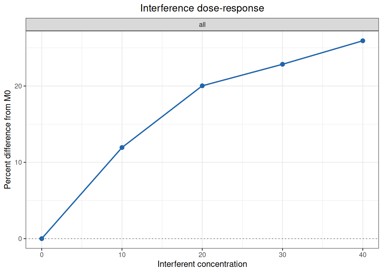

Compare the recalculated values with EP07 Table 4 and Section 6.2.4.3:

EP07 Third Edition Table 4: ivdtools compared with the standard text
Standard location	Statistic	Standard	ivdtools
0	mean	200.020	200.02000
10	mean	223.900	223.90000
20	mean	240.080	240.08000
30	mean	245.720	245.72000
40	mean	251.880	251.88000
0	cv_percent	0.900	0.88760
10	cv_percent	2.100	2.07502
20	cv_percent	1.400	1.39689
30	cv_percent	1.900	1.94907
40	cv_percent	1.800	1.76870
10	absolute_difference	23.880	23.88000
20	absolute_difference	40.060	40.06000
30	absolute_difference	45.700	45.70000
40	absolute_difference	51.860	51.86000
10	percent_difference	11.940	11.93881
20	percent_difference	20.030	20.02800
30	percent_difference	22.850	22.84772
40	percent_difference	25.930	25.92741
all	interference_at_10_percent	8.375	8.37605

Reverse interpolation gives 8.376 mg/dL. The main text reports 8.375 mg/dL when calculated from the rounded 11.94% value in the table, and recommends reporting at most one decimal place after considering study uncertainty, or approximately 8.4 mg/dL. The estimate lies within the measured range but remains an estimate between two nodes; for a critical claim, samples should be prepared and tested near this concentration.

EP07 Section 6.2.5.4 also uses these data to illustrate the limitation of a quadratic curve. Following the main text, fit a quadratic polynomial to all 25 individual results:

Code

ep07_table4_quadratic <- lm(
  result ~ concentration + I(concentration^2),
  data = ep07_table4
)
ep07_table4_quadratic_coef <- coef(ep07_table4_quadratic)

                term     estimate
1        (Intercept) 200.64342857
2      concentration   2.56911429
3 I(concentration^2)  -0.03284286

Quadratic-curve recalculation for EP07 Section 6.2.5.4
Standard location	Statistic	Standard	ivdtools
EP07 6.2.5.4	intercept	200.640000	200.643429
EP07 6.2.5.4	linear_term	2.569100	2.569114
EP07 6.2.5.4	quadratic_term	-0.032843	-0.032843
EP07 6.2.5.4	turning_point	39.100000	39.112223

The quadratic model suggests that the effect turns downward after approximately 39.1 mg/dL. This is mainly a shape imposed by the function, not a mechanism demonstrated by the experiment. The quadratic fit is therefore retained here to reproduce the warning in the standard text, while interpretation continues to use the point-to-point result.

7.4.4 CLSI EP07 Third Edition Table 5: Linear Dose–Response

Table 5 uses the same five interferent concentrations and five measurements per concentration, but the data follow an approximately linear trajectory. In this case, method = “linear” fits the analyte result against interferent concentration using all 25 individual results, rather than regressing only the five concentration means.

Code

ep07_table5 <- read_csv(
  "./data/007-干扰研究/std-ep07-table5-dose-response.csv",
  show_col_types = FALSE
)
head(ep07_table5, 6)

# A tibble: 6 × 6
  sample replicate concentration result concentration_unit result_unit
   <dbl>     <dbl>         <dbl>  <dbl> <chr>              <chr>      
1      1         1             0   200. mg/dL              nmol/L     
2      1         2             0   200. mg/dL              nmol/L     
3      1         3             0   203. mg/dL              nmol/L     
4      1         4             0   198. mg/dL              nmol/L     
5      1         5             0   206. mg/dL              nmol/L     
6      2         1            10   212. mg/dL              nmol/L

Code

ep07_table5_result <- interference_dose_response(
  ep07_table5,
  result = "result",
  concentration = "concentration",
  baseline = 0,
  method = "linear"
)
ep07_table5_result

Interference dose-response analysis
  Method: linear
  Baseline concentration: 0
  Stratum: all | Concentration: 0
    Observations        : 5
    Mean                : 201.44
    SD                  : 3.1101447
    SE                  : 1.390899
    Absolute difference : 0
    Percent difference  : 0
    CV percent          : 1.5439559

  Stratum: all | Concentration: 10
    Observations        : 5
    Mean                : 212.28
    SD                  : 2.2785961
    SE                  : 1.0190191
    Absolute difference : 10.84
    Percent difference  : 5.381255
    CV percent          : 1.0733918

  Stratum: all | Concentration: 20
    Observations        : 5
    Mean                : 226.56
    SD                  : 5.2122932
    SE                  : 2.3310084
    Absolute difference : 25.12
    Percent difference  : 12.470214
    CV percent          : 2.3006237

  Stratum: all | Concentration: 30
    Observations        : 5
    Mean                : 239.2
    SD                  : 2.9597297
    SE                  : 1.3236314
    Absolute difference : 37.76
    Percent difference  : 18.745036
    CV percent          : 1.2373452

  Stratum: all | Concentration: 40
    Observations        : 5
    Mean                : 249.6
    SD                  : 2.9732137
    SE                  : 1.3296616
    Absolute difference : 48.16
    Percent difference  : 23.907863
    CV percent          : 1.1911914

Code

plot(ep07_table5_result, type = "absolute")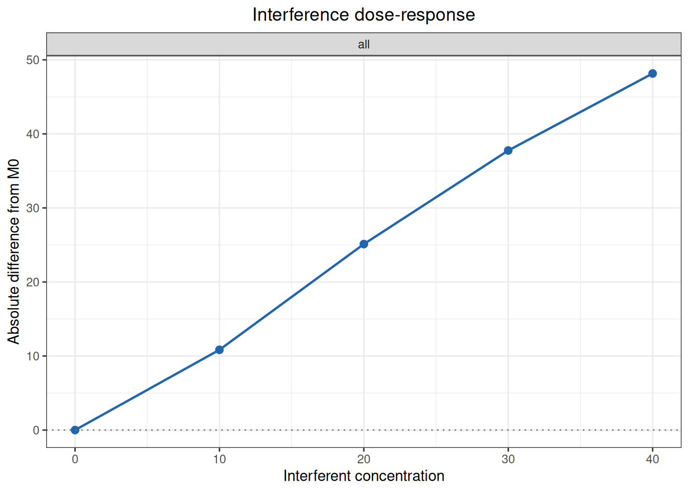

EP07 Third Edition Table 5: ivdtools compared with the standard text
Standard location	Statistic	Standard	ivdtools
0	mean	201.4400	201.44000
10	mean	212.2800	212.28000
20	mean	226.5600	226.56000
30	mean	239.2000	239.20000
40	mean	249.6000	249.60000
0	cv_percent	1.5000	1.54396
10	cv_percent	1.1000	1.07339
20	cv_percent	2.3000	2.30062
30	cv_percent	1.2000	1.23735
40	cv_percent	1.2000	1.19119
all	intercept	201.1700	201.16800
all	slope	1.2324	1.23240
all	difference_intercept	-0.2720	-0.27200

Using the five replicates at 0 mg/dL gives \(M_0=201.44\) nmol/L. Regression of all individual results gives \(Y=1.2324X+201.168\); the main text writes the intercept as 201.17 nmol/L. If the results are first converted to absolute effects using \(M_0\), the equation is \(d=1.2324X-0.272\). The regression intercept and the measured baseline mean are two different estimates of the no-interferent result and should not be mixed. The linear method is appropriate only when the scatter is approximately linear across the measured range; a high goodness of fit does not justify ignoring local curvature or extrapolating beyond the observed range.

7.4.5 YY/T 1789.5–2023 Appendix A: Interferent-Spike Screening

Appendix A uses low- and high-level thyroid-stimulating hormone (TSH) samples, at 0.3 and 5.0 µIU/mL, respectively. It screens 2,000 mg/dL hemoglobin and 2,000 IU/mL rheumatoid factor. Test preparations receive interferent stock solution, while control preparations receive the same volume of physiological saline; each preparation is measured three times.

Code

yyt1789_a_data <- read_csv(
  "./data/007-干扰研究/std-yyt1789-5-appendix-a-paired.csv",
  show_col_types = FALSE
)
head(yyt1789_a_data, 6)

# A tibble: 6 × 7
  interferent analyte_level condition interferent_concentration replicate result
  <chr>       <chr>         <chr>                         <dbl>     <dbl>  <dbl>
1 hemoglobin  low           control                           0         1  0.272
2 hemoglobin  low           control                           0         2  0.279
3 hemoglobin  low           control                           0         3  0.278
4 hemoglobin  low           test                           2000         1  0.347
5 hemoglobin  low           test                           2000         2  0.358
6 hemoglobin  low           test                           2000         3  0.354
# ℹ 1 more variable: unit <chr>

Code

yyt1789_a <- interference_paired(
  yyt1789_a_data,
  result = "result",
  design = "ep07",
  condition = "condition",
  test_level = "test",
  control_level = "control",
  by = c("interferent", "analyte_level"),
  conf.level = 0.95
)

Code

plot(yyt1789_a)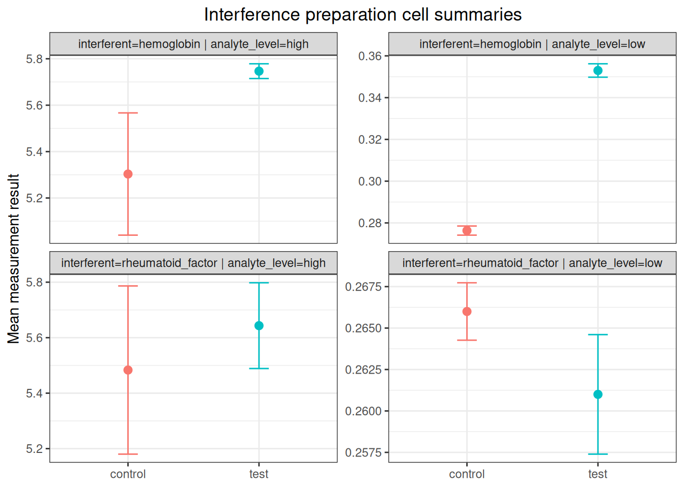

Compare the results with the standard text:

YY/T 1789.5 Appendix A: ivdtools compared with the standard text
Standard location	Statistic	Standard	ivdtools
hemoglobin_low	control_mean	0.276	0.2763
hemoglobin_low	test_mean	0.353	0.3530
hemoglobin_low	difference	0.077	0.0767
hemoglobin_high	control_mean	5.303	5.3033
hemoglobin_high	test_mean	5.747	5.7467
hemoglobin_high	difference	0.443	0.4433
rheumatoid_factor_low	control_mean	0.266	0.2660
rheumatoid_factor_low	test_mean	0.261	0.2610
rheumatoid_factor_low	difference	-0.005	-0.0050
rheumatoid_factor_high	control_mean	5.483	5.4833
rheumatoid_factor_high	test_mean	5.643	5.6433
rheumatoid_factor_high	difference	0.160	0.1600

The hemoglobin effects at the low and high levels are 0.0767 and 0.4433 µIU/mL, respectively. The critical bias values \(B_c\) in Table A.3 are 0.024 and 0.432 µIU/mL, so both levels proceed to further dose–response evaluation under the statistical rule in the standard text. The rheumatoid-factor effects are −0.0050 and 0.1600 µIU/mL, within the case’s technical limits of ±0.03 and ±0.5 µIU/mL, respectively.

The confidence intervals from the paired-interference analysis use the observed SD of the preparation units. Table A.3 of YY/T 1789.5 instead uses the repeatability SD from a prior precision study and a standard-specific formula for \(B_c\). This case therefore compares preparation-unit means and effects with the standard table without misrepresenting the software interval as the standard’s \(B_c\) decision.

7.4.6 YY/T 1789.5–2023 Appendix B: Hemoglobin Dose–Response

Appendix B prepares low- and high-level TSH samples at five hemoglobin concentrations: 0, 500, 1,000, 1,500, and 2,000 mg/dL, with three measurements at each concentration. The standard uses the mean at 0 mg/dL as the control and uses point-to-point interpolation to determine the interferent concentration at which the allowable bias is reached.

Code

yyt1789_b_data <- read_csv(
  "./data/007-干扰研究/std-yyt1789-5-appendix-b-dose.csv",
  show_col_types = FALSE
)
head(yyt1789_b_data, 6)

# A tibble: 6 × 7
  interferent analyte_level concentration replicate result result_unit
  <chr>       <chr>                 <dbl>     <dbl>  <dbl> <chr>      
1 hemoglobin  low                       0         1  0.282 uIU/mL     
2 hemoglobin  low                       0         2  0.29  uIU/mL     
3 hemoglobin  low                       0         3  0.263 uIU/mL     
4 hemoglobin  low                     500         1  0.274 uIU/mL     
5 hemoglobin  low                     500         2  0.307 uIU/mL     
6 hemoglobin  low                     500         3  0.31  uIU/mL     
# ℹ 1 more variable: concentration_unit <chr>

Code

yyt1789_b <- interference_dose_response(
  yyt1789_b_data,
  result = "result",
  concentration = "concentration",
  by = "analyte_level",
  baseline = 0,
  method = "point_to_point"
)

The allowable bias for the low-level sample is ±0.03 µIU/mL. Reverse-interpolate the absolute effect at 0.03 µIU/mL:

Code

yyt1789_b_limit <- predict(
  yyt1789_b,
  target = 0.03,
  metric = "absolute",
  stratum = "analyte_level=low"
)

Code

plot(yyt1789_b, type = "absolute")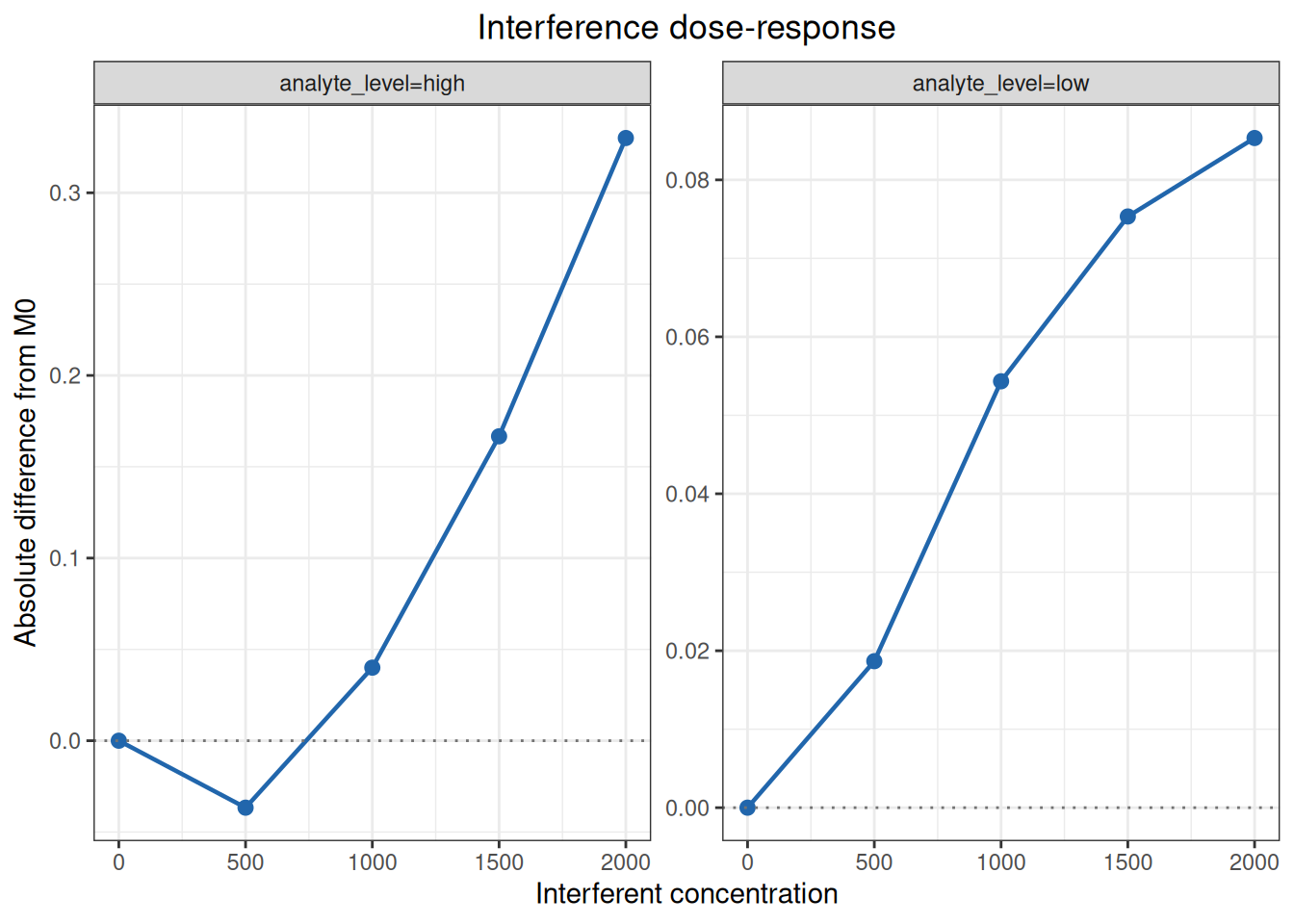

Compare the results with the standard text:

YY/T 1789.5 Appendix B: ivdtools compared with the standard text
Standard location	Statistic	Standard	ivdtools
low_0	mean	0.278	0.2783
low_0	difference	0.000	0.0000
low_500	mean	0.297	0.2970
low_500	difference	0.019	0.0187
low_1000	mean	0.333	0.3327
low_1000	difference	0.054	0.0543
low_1500	mean	0.354	0.3537
low_1500	difference	0.075	0.0753
low_2000	mean	0.364	0.3637
low_2000	difference	0.085	0.0853
high_0	mean	5.273	5.2733
high_0	difference	0.000	0.0000
high_500	mean	5.237	5.2367
high_500	difference	-0.037	-0.0367
high_1000	mean	5.313	5.3133
high_1000	difference	0.040	0.0400
high_1500	mean	5.440	5.4400
high_1500	difference	0.167	0.1667
high_2000	mean	5.603	5.6033
high_2000	difference	0.330	0.3300
low	interference_concentration	658.880	658.8785

The low-level effect crosses 0.03 µIU/mL between 500 and 1,000 mg/dL, giving 658.88 mg/dL by point-to-point reverse interpolation. At the high level, the absolute effect remains within ±0.5 µIU/mL at all measured concentrations. The case therefore reports 658.88 mg/dL as the hemoglobin concentration resisted by the evaluated system, taking the lower result of the two analyte levels. This is an interpolation between measured nodes, not a result measured directly at 658.88 mg/dL.

7.4.7 YY/T 1789.5–2023 Appendix C: Patient-Sample Evaluation

Appendix C uses EDTA-anticoagulated plasma as the test group and serum as the control group, with 20 patient samples in each group. Every sample is measured by both the evaluated measurement procedure and a comparative procedure claimed for serum and EDTA plasma. The source Table C.1 lists one procedure result per sample, rather than single-replicate records, so the input has one row per sample-by-procedure combination.

Code

yyt1789_c_data <- read_csv(
  "./data/007-干扰研究/std-yyt1789-5-appendix-c-patient.csv",
  show_col_types = FALSE
)
head(yyt1789_c_data, 6)

# A tibble: 6 × 5
  id    group   method      result unit  
  <chr> <chr>   <chr>        <dbl> <chr> 
1 C01   control comparative  23.3  uIU/mL
2 C01   control evaluated    23.5  uIU/mL
3 C02   control comparative   8    uIU/mL
4 C02   control evaluated     2.73 uIU/mL
5 C03   control comparative   5.35 uIU/mL
6 C03   control evaluated     4.47 uIU/mL

Code

yyt1789_c <- interference_patient(
  yyt1789_c_data,
  id = "id",
  group = "group",
  method = "method",
  result = "result",
  test_group = "test",
  control_group = "control",
  evaluated_method = "evaluated",
  comparative_method = "comparative",
  conf.level = 0.95
)
yyt1789_c

Patient-specimen interference evaluation
  Evaluated - comparative: evaluated - comparative
  Group: test
    Observations            : 20
    Mean difference         : -1.1835
    SD difference           : 2.3930541
    SE difference           : 0.53510317
    Median difference       : -0.49
    25th percentile         : -1.3425
    75th percentile         : -0.32
    CI lower                : -2.3034838
    CI upper                : -0.063516183
    Mean percent difference : -17.916419
    SD percent difference   : 18.774944
    Percent CI lower        : -26.703363
    Percent CI upper        : -9.1294749

  Group: control
    Observations            : 20
    Mean difference         : -1.039
    SD difference           : 2.1614978
    SE difference           : 0.4833256
    Median difference       : -0.415
    25th percentile         : -0.835
    75th percentile         : -0.075
    CI lower                : -2.0506121
    CI upper                : -0.027387902
    Mean percent difference : -11.712959
    SD percent difference   : 24.21947
    Percent CI lower        : -23.04802
    Percent CI upper        : -0.37789805

Code

plot(yyt1789_c, type = "difference")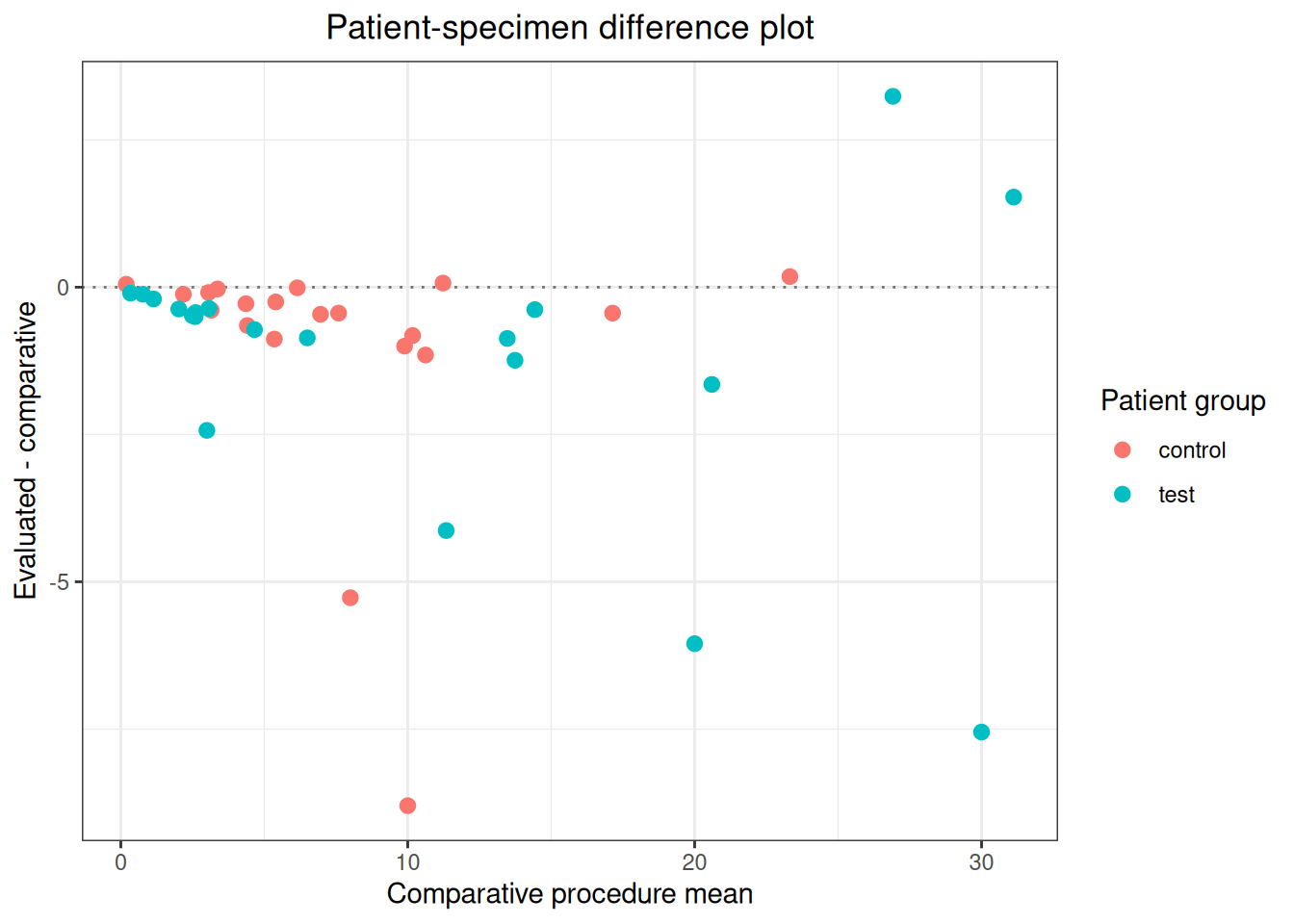

Compare the results with the standard text:

YY/T 1789.5 Appendix C: ivdtools compared with the standard text
Standard location	Statistic	Standard	ivdtools
control	mean_difference	-1.04	-1.0390
control	sd_difference	2.16	2.1615
control	ci_lower	-2.05	-2.0506
control	ci_upper	-0.03	-0.0274
test	mean_difference	-1.18	-1.1835
test	sd_difference	2.39	2.3931
test	ci_lower	-2.30	-2.3035
test	ci_upper	-0.06	-0.0635

The mean difference for the control group is −1.039 µIU/mL, with a 95% CI of −2.051 to −0.027 µIU/mL. For the test group, the mean is −1.184 µIU/mL, with a 95% CI of −2.303 to −0.064 µIU/mL. The intervals overlap, so Appendix C concludes that the EDTA anticoagulant does not interfere with this TSH measurement. Both groups show negative bias relative to the comparative procedure; the decision is based on overlap between the two group intervals, not on whether either interval contains zero.

7.4.8 YY/T 1789.5–2023 Appendix D: Cross-Reactivity Evaluation

Appendix D adds 200,000 µIU/mL luteinizing hormone (LH) to low- and high-level TSH base samples and uses controls with the same volume of diluent. First obtain the test-minus-control effect with paired interference analysis, then calculate the standard-defined cross-reactivity rate:

\[\text{Cross-reactivity rate}=\frac{\bar{x}_{T}-\bar{x}_{C}}{C_{interferent}}\times100\%.\]

Code

yyt1789_d_data <- read_csv(
  "./data/007-干扰研究/std-yyt1789-5-appendix-d-cross-reactivity.csv",
  show_col_types = FALSE
)
head(yyt1789_d_data)

# A tibble: 6 × 8
  interferent analyte_level condition interferent_concentration replicate result
  <chr>       <chr>         <chr>                         <dbl>     <dbl>  <dbl>
1 LH          low           control                           0         1  0.281
2 LH          low           control                           0         2  0.283
3 LH          low           control                           0         3  0.282
4 LH          low           test                         200000         1  0.312
5 LH          low           test                         200000         2  0.305
6 LH          low           test                         200000         3  0.298
# ℹ 2 more variables: result_unit <chr>, concentration_unit <chr>

Code

yyt1789_d <- interference_paired(
  yyt1789_d_data,
  result = "result",
  design = "ep07",
  condition = "condition",
  test_level = "test",
  control_level = "control",
  by = "analyte_level",
  conf.level = 0.95
)
yyt1789_d

Interference paired-difference analysis
  Design: ep07
  Confidence level: 95%
  analyte_level: low
    stratum             : analyte_level=low
    design              : ep07
    n_test              : 3
    n_control           : 3
    test_mean           : 0.305
    control_mean        : 0.282
    absolute_difference : 0.023
    absolute_se         : 0.0040824829
    df                  : 4
    absolute_ci_lower   : 0.01166521
    absolute_ci_upper   : 0.03433479
    percent_difference  : 8.1560284
    percent_se          : 1.447689
    percent_ci_lower    : 4.1365994
    percent_ci_upper    : 12.175457

  analyte_level: high
    stratum             : analyte_level=high
    design              : ep07
    n_test              : 3
    n_control           : 3
    test_mean           : 5.2366667
    control_mean        : 5.04
    absolute_difference : 0.19666667
    absolute_se         : 0.04772607
    df                  : 4
    absolute_ci_lower   : 0.064157853
    absolute_ci_upper   : 0.32917548
    percent_difference  : 3.9021164
    percent_se          : 0.94694584
    percent_ci_lower    : 1.2729733
    percent_ci_upper    : 6.5312595

Code

yyt1789_d_effects <- yyt1789_d$effects
yyt1789_d_effects$cross_reactivity_percent <-
  100 * yyt1789_d_effects$absolute_difference / 200000

Compare the results with the standard text:

YY/T 1789.5 Appendix D: ivdtools compared with the standard text
Standard location	Statistic	Standard	ivdtools
low	control_mean	0.28200	0.282000
low	test_mean	0.30500	0.305000
low	cross_reactivity_percent	0.00001	0.000012
high	control_mean	5.04000	5.040000
high	test_mean	5.24000	5.236667
high	cross_reactivity_percent	0.00010	0.000098

The cross-reactivity rates for the low- and high-level samples are approximately 0.00001% and 0.00010%, respectively, both within the case’s prespecified range of −0.1% to 0.1%. This conversion is appropriate only when the unit relationship between analyte result and interferent concentration has a clear scientific meaning. The report must state both units and the interferent concentration used in the experiment.

7.5 Detailed Function Reference

7.5.1 Replicate Planning with interference_replicates()

Code

interference_replicates(
  sd,
  detectable_difference,
  alpha = 0.05,
  power = 0.90,
  alternative = c("two.sided", "one.sided"),
  min_replicates = 5L,
  label = NULL
)

sd is expected repeatability SD; for relative-scale planning it is repeatability CV. detectable_difference uses the same scale and a compatible length. alpha is the type-I error probability, power is the target power, alternative selects a two- or one-sided design, min_replicates is the minimum number of test and control replicates per preparation, and label optionally names each calculation.

The result is an interference_replicates data frame with one row per design. It includes the inputs, difference_over_sd, z_alpha, z_power, calculated_replicates before rounding, and the final replicates_per_sample. The final count applies separately to each test and control preparation.

7.5.2 Paired Preparation with interference_paired()

Code

interference_paired(
  data,
  result,
  design = c("ep07", "analyte_spike", "blank"),
  by = NULL,
  condition = NULL,
  test_level = "test",
  control_level = "control",
  matrix = NULL,
  normal_level = "normal",
  interferent_level = "interferent",
  spike = NULL,
  unspiked_level = "unspiked",
  spiked_level = "spiked",
  conf.level = 0.95
)

data is a long-format data frame with one replicate result per row. result names the numeric measurement column. design can be ep07, analyte_spike, or blank. by optionally supplies stratification columns such as interferent and analyte level. condition identifies test/control conditions for ep07 and optionally blank designs. test_level and control_level identify those values. matrix identifies the matrix column for analyte_spike; normal_level and interferent_level identify normal and interferent matrices; spike identifies analyte-spike status, and unspiked_level and spiked_level identify the two states. conf.level is the effect-interval confidence level.

For ep07, use condition with test_level and control_level. For analyte_spike, use matrix and spike settings. For blank, use condition to distinguish interferent blank and control, or compare with a theoretical zero when no control records exist.

The returned interference_paired object contains effects by stratum, including sample sizes, test/control means, absolute and relative effects, SEs, and intervals. cell_summary contains preparation-unit n, mean, SD, and SE; issues records data problems; excluded_rows stores omitted input rows; analysis_data stores analyzed rows. plot() returns preparation-unit and effect figures.

7.5.3 Dose–Response with interference_dose_response()

Code

interference_dose_response(
  data,
  result,
  concentration,
  by = NULL,
  baseline = 0,
  method = c("point_to_point", "linear"),
  conf.level = 0.95
)

predict(
  object,
  newdata = NULL,
  target = NULL,
  metric = c("result", "absolute", "percent"),
  stratum = NULL
)

plot(x, type = c("response", "absolute", "percent"))

data is a long-format dose-response data frame. result and concentration name the numeric result and interferent concentration columns. by optionally defines strata. baseline is the measured interferent concentration used for the baseline mean and must occur in every stratum. point_to_point interpolates between adjacent concentration means; linear fits a line to individual results. conf.level is the regression-coefficient confidence level.

predict() takes a dose-response object. Supply newdata to predict a result or effect at interferent concentrations, or target to reverse-predict the interferent concentration at a specified result/effect; exactly one of newdata and target is required. metric selects result, absolute effect, or percentage effect; stratum selects one or more strata. The function does not extrapolate and returns missing values outside the observed range. plot() selects result, absolute-effect, or percentage-effect figures.

The returned interference_dose_response object contains a summary of n, mean, SD, SE, CV, absolute effect, and percentage effect at each concentration; diagnostics for baseline, level count, replicate range, and monotonicity; coefficients and models for the linear method; and issues, excluded_rows, and analysis_data. predict() returns stratum, direction, metric, input, estimate, and within_observed_range.

7.5.4 Patient-Sample Comparison with interference_patient()

Code

interference_patient(
  data,
  id,
  group,
  method,
  result,
  test_group,
  control_group,
  evaluated_method,
  comparative_method,
  interferent_cols = NULL,
  conf.level = 0.95
)

plot(
  x,
  type = c("difference", "interferent"),
  interferent = NULL
)

data is a long-format patient-sample result data frame. id names the sample identifier, group the patient test/control group, method the measurement procedure, and result the numeric result. test_group and control_group identify the two patient groups. evaluated_method and comparative_method define the difference direction as evaluated minus comparative. interferent_cols optionally names numeric interferent columns; each is fitted in a separate univariate model. conf.level controls group summaries and regression coefficients.

For plot(), type = “difference” plots method difference against the comparative-procedure mean; type = “interferent” plots difference against a selected interferent concentration. When several interferent columns exist, interferent selects the column to plot.

The returned interference_patient object contains method_summary for sample-by-method n, mean, and SD; specimen_results for complete method pairs and absolute/relative differences; group_summary for group-level differences and intervals; regressions and models for each interferent; and issues, incomplete_ids, and excluded_rows. plot() returns the corresponding figure.