16 Limits of Blank, Detection, and Quantitation

This chapter explains how to turn low-concentration experimental data into auditable sensitivity conclusions for the limit of blank (LoB), limit of detection (LoD), limit of quantitation (LoQ), and verification of those claims. The metrics answer different questions: LoB describes the upper tail of the blank distribution, LoD describes detection capability, and LoQ must additionally specify a precision or total-error requirement.

Workflow: establish or verify LoB, LoD, and LoQ

%%{init: {"theme":"base","themeVariables":{"primaryColor":"#EAF2FB","primaryBorderColor":"#2780E3","primaryTextColor":"#212529","lineColor":"#6C757D","secondaryColor":"#EAF7E6","tertiaryColor":"#FFF4E8","fontSize":"13px"},"flowchart":{"nodeSpacing":18,"rankSpacing":24,"padding":6}}}%%

flowchart LR
    A["Define LoB, LoD, LoQ<br/>or claim-verification objective"] --> B["sensitivity_design()<br/>Check design"]
    B --> C["sensitivity_lob()"]
    C --> D["sensitivity_lod()"]
    D --> E["sensitivity_loq()"]
    E --> F["sensitivity_verify()"]
    F --> G["Check method, precision profile,<br/>and verification rate"]

    classDef input fill:#EAF2FB,stroke:#2780E3,color:#212529
    classDef process fill:#EAF7E6,stroke:#3FB618,color:#212529
    classDef output fill:#F4EEFB,stroke:#9954BB,color:#212529
    class A input
    class B,C,D,E,F process
    class G output

Code

library(ivdtools)

16.1 Main Functions

The analytical-sensitivity module uses raw long-format data as its main input and separates limit establishment, claim verification, and study design:

Function	Purpose
`sensitivity_lob()`	Establish nonparametric, parametric, or zero LoB
`sensitivity_lod()`	Classical, nonparametric, precision-profile, or Probit LoD
`sensitivity_loq()`	Westgard, RMS, precision-based, or custom-target LoQ
`sensitivity_verify()`	Verify an existing LoB, LoD, or LoQ claim
`sensitivity_design()`	View minimum design requirements and actual data counts

16.1.1 Interfaces, Parameters, and Core Statistics

Code

sensitivity_lob(
  data, result, sample, lot = NULL,
  method = c("nonparametric", "parametric", "zero"),
  alpha = 0.05, lot_rule = c("ep17", "separate", "combined"),
  exclude = NULL
)
sensitivity_lod(
  data, result = NULL, sample = NULL, lob, lot = NULL,
  concentration = NULL, detected = NULL,
  method = c("classical", "nonparametric", "profile", "probit"),
  beta = 0.05, profile_model = c("linear", "quadratic", "sadler", "vfp")
)
sensitivity_loq(
  data, result, sample, assigned, lot = NULL,
  method = c("westgard", "rms", "precision", "custom"),
  goal, goal_scale = c("relative", "absolute"),
  lod = NULL, k = 2, profile = FALSE
)

Nonparametric LoB is the \((1-\alpha)\) rank quantile of blank results; the parametric method uses

\[ LoB=\bar x_B+c_p s_B, \]

where \(c_p\) applies a finite-sample correction based on \(α\) and blank degrees of freedom \(B-K\). method="zero" fixes \(LoB=0\) and reports the proportion of blank results above zero. For classical LoD, SDs from multiple low-level samples are pooled by degrees of freedom:

\[ s_p=\sqrt{\frac{\sum_j(n_j-1)s_j^2}{\sum_j(n_j-1)}}, \]

and combined with LoB, \(β\), and a finite-sample correction. The precision-profile method solves for concentration-dependent SD; the Probit method fits the detection-probability–concentration relationship. Their data structures and assumptions differ.

At each LoQ level, bias is \(b=\bar x-x_a\). The four error quantities are:

`method`	Quantity compared with `goal`
`westgard`	\(\|b\|+k s\)
`rms`	\(\sqrt{s^2+b^2}\)
`precision`	\(s\)
`custom`	Value returned by `accuracy_function()`

When goal_scale="relative", the quantity is divided by \(|x_a|\). A candidate LoQ is the lowest observed mean or fitted-profile intersection satisfying the target. Multiple lots are handled by the selected lot_rule, and the most conservative finite candidate is reported. When LoD is supplied,

\[ LoQ_{\mathrm{reported}}=\max(LoQ_{\mathrm{candidate}},LoD). \]

sensitivity_lob(), sensitivity_lod(), and sensitivity_loq() return the corresponding limit, method, core statistics, and diagnostics.

16.1.2 Claim Verification and Design Checks

Code

sensitivity_verify(
  data, result, sample, limit = c("lob", "lod", "loq"),
  claim, lob = NULL, assigned = NULL, allowable_error = NULL,
  error_scale = c("relative", "absolute"), alpha = 0.05
)
sensitivity_design(method = "all", data = NULL, ...)

LoB verification counts \(x\le claim\), LoD verification counts \(x\ge LoB\), and LoQ verification checks whether results fall within the allowable-error window around the assigned value. The function returns the observed success proportion, a one-sided Wilson score interval, and EP17 Table 1 boundaries, but intentionally does not generate a pass field. sensitivity_design() gives minimum design requirements and can summarize actual data counts; it shows gaps but does not replace protocol decisions.

sensitivity_verify() returns the observed success proportion, Wilson interval, and boundary information. sensitivity_design() returns minimum requirements and an actual-count table.

16.2 Analysis Examples

16.2.1 LoB

Each row of the raw data is one measurement:

Code

# Simulate data
set.seed(17)
blank <- expand.grid(
  lot = c("A", "B"), sample = paste0("blank", 1:4), replicate = 1:15
)
blank$result <- rnorm(nrow(blank), 0.2, 0.1)
head(blank, 6)

  lot sample replicate     result
1   A blank1         1 0.09849913
2   B blank1         1 0.19203633
3   A blank2         1 0.17670130
4   B blank2         1 0.11827321
5   A blank3         1 0.27720908
6   B blank3         1 0.18343881

Code

# Establish LoB
lob_np <- sensitivity_lob(
  blank, result = "result", sample = "sample", lot = "lot",
  method = "nonparametric"
)
lob_np

Analytical sensitivity: LOB 
  Method: nonparametric 
  Estimate: 0.378828

EP17 lot rules are used by default for all establishment functions: 2–3 lots are calculated separately and the maximum is reported; 4 or more lots are combined. Negative measurement results are not automatically truncated to 0.

16.2.2 LoD

Classical LoD uses the pooled SD of low-level samples:

Code

# Simulate data
low <- expand.grid(
  lot = c("A", "B"), sample = paste0("low", 1:4), replicate = 1:15
)
low$result <- rnorm(nrow(low), 1.2, 0.2)
head(low, 6)

  lot sample replicate    result
1   A   low1         1 1.4763513
2   B   low1         1 1.2897865
3   A   low2         1 1.1695380
4   B   low2         1 1.2518588
5   A   low3         1 0.8777197
6   B   low3         1 0.7982088

Code

# Establish LoD
lod_classical <- sensitivity_lod(
  low, result = "result", sample = "sample", lot = "lot",
  lob = lob_np, method = "classical"
)
lod_classical

Analytical sensitivity: LOD 
  Method: classical 
  Estimate: 0.771614

method = "profile" supports linear, quadratic, sadler, and vfp precision profiles; method = "probit" supports raw 0/1 detection results or count/total summaries. Cochran statistics and fit measures are diagnostics only; the program does not choose the analysis path for the user.

16.2.3 LoQ

The LoQ accuracy target must be prespecified. A relative target is expressed as a proportion, so 21.6% is written 0.216:

Code

# Simulate data
loq_data <- expand.grid(
  lot = c("A", "B"), sample = paste0("pool", 1:4), replicate = 1:9
)
loq_data$assigned <- rep(rep(c(30, 35, 40, 45), each = 9), 2)
loq_data$result <- rnorm(nrow(loq_data), loq_data$assigned,
                         0.06 * loq_data$assigned)
head(loq_data, 6)

  lot sample replicate assigned   result
1   A  pool1         1       30 29.70842
2   B  pool1         1       30 28.62287
3   A  pool2         1       30 29.82049
4   B  pool2         1       30 30.07043
5   A  pool3         1       30 28.84843
6   B  pool3         1       30 28.98056

Code

# Establish LoQ
loq_te <- sensitivity_loq(
  loq_data, result = "result", sample = "sample", assigned = "assigned",
  lot = "lot", method = "westgard", goal = 0.216,
  goal_scale = "relative", lod = lod_classical
)
loq_te

Analytical sensitivity: LOQ 
  Method: westgard 
  Estimate: 29.4924 
  Candidate LoQ: 29.4924 
  Reported LoQ : 29.4924

The result stores both candidate_loq and reported_loq, so the LoD constraint does not overwrite the original candidate value.

16.2.4 Claim Verification

limit can specify only one claim type at a time:

Code

# Simulate data
verification <- data.frame(
  sample = rep(c("blank1", "blank2"), each = 10),
  result = c(rep(0, 19), 1.2)
)
head(verification, 6)

  sample result
1 blank1      0
2 blank1      0
3 blank1      0
4 blank1      0
5 blank1      0
6 blank1      0

Code

# Verify LoB
v_lob <- sensitivity_verify(
  verification, result = "result", sample = "sample",
  limit = "lob", claim = 1
)
v_lob

Analytical sensitivity: VERIFICATION 
  Method: lob 
  Limit                    : lob
  Claim                    : 1
  LoB                      : 1
  Total results            : 20
  Consistent results       : 19
  Observed proportion      : 0.95
  Score CI lower           : 0.80399276
  Score CI upper           : 0.98876518
  EP17 boundary            : 0.85
  Difference from boundary : 0.1

LoB: count result <= claim.
LoD: count result >= lob; the LoD claim is not a detection decision threshold.
LoQ: check whether the result falls within the allowable-error window around each sample’s assigned value.

The result contains the observed proportion, one-sided Wilson interval, EP17 Table 1 boundaries, and differences. It does not contain a pass or verified field.

16.2.5 Study Design

Code

sensitivity_design("all")

Analytical sensitivity study design
  Method: classical
    Reagent lots         : 2
    Instruments          : 1
    Days                 : 3
    Blank samples        : 4
    Low samples          : 4
    Concentration levels : NA
    Replicates per lot   : 60
    Replicate scope      : blank and low results separately

  Method: profile
    Reagent lots         : 2
    Instruments          : 1
    Days                 : 5
    Blank samples        : 0
    Low samples          : 5
    Concentration levels : 5
    Replicates per lot   : 40
    Replicate scope      : per sample

  Method: probit
    Reagent lots         : 2
    Instruments          : NA
    Days                 : NA
    Blank samples        : 0
    Low samples          : 3
    Concentration levels : 5
    Replicates per lot   : 20
    Replicate scope      : per sample and concentration level

  Method: loq
    Reagent lots         : 2
    Instruments          : 1
    Days                 : 3
    Blank samples        : 0
    Low samples          : 4
    Concentration levels : 1
    Replicates per lot   : 36
    Replicate scope      : total low results

  Method: verification
    Reagent lots         : 1
    Instruments          : 1
    Days                 : 3
    Blank samples        : 2
    Low samples          : 0
    Concentration levels : 1
    Replicates per lot   : 20
    Replicate scope      : total verification results

Code

sensitivity_design("verification", verification,
                   result = "result", sample = "sample", limit = "lob")

Analytical sensitivity study design
  Method               : verification
  Reagent lots         : 1
  Instruments          : 1
  Days                 : 3
  Blank samples        : 2
  Low samples          : 0
  Concentration levels : 1
  Replicates per lot   : 20
  Replicate scope      : total verification results

Observed study counts
  Observations         : 20
  Reagent lots         : NA
  Days                 : NA
  Samples              : 2
  Concentration levels : NA

The design object reports minimum requirements alongside actual counts but does not make a pass/fail decision. Exclusions must be supplied explicitly through exclude and are preserved in the result object.

16.2.6 Standard Case: CLSI EP17-A2 Appendix A, Classical LoB and LoD

Two reagent lots each have 60 blank and 60 low-level results. Calculate each lot under the EP17 lot rule and report the larger value.

Code

ep17_blank <- read.csv("./data/016-分析灵敏度/std-ep17-appendix-a-blank.csv", check.names = FALSE)
ep17_low <- read.csv("./data/016-分析灵敏度/std-ep17-appendix-a-low.csv", check.names = FALSE)

ep17_lob_np <- sensitivity_lob(
  ep17_blank, result = "result", sample = "sample", lot = "lot",
  method = "nonparametric"
)
ep17_lod_np <- sensitivity_lod(
  ep17_low, result = "result", sample = "sample", lot = "lot",
  lob = ep17_lob_np, method = "classical"
)
ep17_lob_p <- sensitivity_lob(
  ep17_blank, result = "result", sample = "sample", lot = "lot",
  method = "parametric"
)
ep17_lod_p <- sensitivity_lod(
  ep17_low, result = "result", sample = "sample", lot = "lot",
  lob = ep17_lob_p, method = "classical"
)

EP17-A2 Appendix A: comparison with the standard
Standard position	Statistic	Standard result	ivdtools result
EP17-A2 Appendix A	nonparametric LoB lot 1	7.6	7.6000
EP17-A2 Appendix A	nonparametric LoB lot 2	9.4	9.4000
EP17-A2 Appendix A	nonparametric LoB report	9.4	9.4000
EP17-A2 Appendix A	classical LoD lot 1	14.5	14.5309
EP17-A2 Appendix A	classical LoD lot 2	13.8	13.8343
EP17-A2 Appendix A	classical LoD report	14.5	14.5309
EP17-A2 Appendix A	parametric LoB report	8.8	8.7956
EP17-A2 Appendix A	parametric LoD report	13.9	13.9266

Negative measurement results are retained as in the source table and are not truncated to 0.

16.2.7 Standard Case: CLSI EP17-A2 Appendix C, Probit LoD

All 66 zero-concentration results from three lots are negative, supporting LoB = 0 in this example. Because zero concentration cannot be log-transformed, only positive-concentration rows are sent to the Probit model; zero-concentration counts remain in the input table for LoB checking.

Code

ep17_probit <- read.csv("./data/016-分析灵敏度/std-ep17-appendix-c-probit.csv", check.names = FALSE)
ep17_probit_fit_data <- ep17_probit[ep17_probit$concentration > 0, ]

ep17_c_lod <- sensitivity_lod(
  ep17_probit_fit_data,
  result = "positive", sample = "sample", lob = 0, lot = "lot",
  concentration = "concentration", detected = "positive", total = "total",
  method = "probit", concentration_scale = "log10"
)
plot(ep17_c_lod)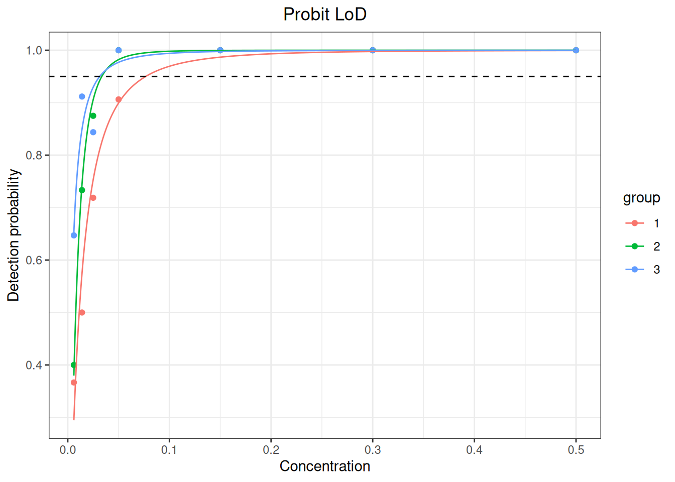

EP17-A2 Appendix C: comparison with the standard
Standard position	Statistic	Standard result	ivdtools result
EP17-A2 Appendix C	Probit LoD lot 1	0.077	0.0766
EP17-A2 Appendix C	Probit LoD lot 2	0.033	0.0335
EP17-A2 Appendix C	Probit LoD lot 3	0.031	0.0314

The three LoDs are 0.077, 0.033, and 0.031 CFU/mL; the maximum, 0.077 CFU/mL, is reported. Neither goodness-of-fit test indicates lack of fit, but this appendix uses one sample, a deliberate simplification that falls below the minimum three-sample design and must not be treated as a compliant study template.

16.2.8 Standard Case: CLSI EP17-A2 Appendices E and F, Claim Verification

Code

ep17_ef <- read.csv("./data/016-分析灵敏度/std-ep17-appendix-e-verification.csv", check.names = FALSE)
ep17_f <- read.csv("./data/016-分析灵敏度/std-ep17-appendix-f-loq-verification.csv", check.names = FALSE)

ep17_verify_lob <- sensitivity_verify(
  ep17_ef[ep17_ef$type == "blank", ],
  result = "result", sample = "sample", limit = "lob", claim = 20
)
ep17_verify_lod <- sensitivity_verify(
  ep17_ef[ep17_ef$type == "positive", ],
  result = "result", sample = "sample", limit = "lod", claim = 45,
  lob = 20
)
ep17_verify_loq <- sensitivity_verify(
  ep17_f, result = "result", sample = "sample", limit = "loq", claim = 50,
  assigned = "target", allowable_error = 0.15
)

EP17-A2 Appendices E-F: comparison with the standard
Standard position	Statistic	Standard result	ivdtools result
EP17-A2 Appendices E-F	LoB consistency (%)	95.8	95.8333
EP17-A2 Appendices E-F	LoD consistency (%)	91.7	91.6667
EP17-A2 Appendices E-F	LoQ consistency (%)	91.1	91.1111

16.2.9 Standard Case: YY/T 1789.3-2022 Appendix A, ProGRP

Appendix A gives 60 blank and 60 low-concentration results for each of two lots and can be analyzed directly with sensitivity_lob() and sensitivity_lod(). Negative blanks are retained as reported and are not truncated to zero.

Code

yyt1789_3_blank <- read.csv(
  "./data/016-分析灵敏度/std-yyt1789-3-appendix-a-blank.csv"
)
yyt1789_3_low <- read.csv(
  "./data/016-分析灵敏度/std-yyt1789-3-appendix-a-low.csv"
)

yyt1789_3_lob_np <- sensitivity_lob(
  yyt1789_3_blank, result = "result", sample = "sample", lot = "lot",
  method = "nonparametric"
)
yyt1789_3_lob_p <- sensitivity_lob(
  yyt1789_3_blank, result = "result", sample = "sample", lot = "lot",
  method = "parametric"
)
yyt1789_3_lod_classical <- sensitivity_lod(
  yyt1789_3_low, result = "result", sample = "sample", lot = "lot",
  lob = yyt1789_3_lob_np, method = "classical"
)
yyt1789_3_lod_np <- sensitivity_lod(
  yyt1789_3_low, result = "result", sample = "sample", lot = "lot",
  lob = yyt1789_3_lob_np, method = "nonparametric"
)

YY/T 1789.3-2022 Appendix A: comparison with the standard
Standard position	Statistic	Standard result	ivdtools result
YY/T 1789.3 Appendix A	nonparametric LoB lot 1	0.240	0.2450
YY/T 1789.3 Appendix A	nonparametric LoB lot 2	0.250	0.2500
YY/T 1789.3 Appendix A	reported LoB	0.250	0.2500
YY/T 1789.3 Appendix A	parametric LoB lot 1	0.174	0.1758
YY/T 1789.3 Appendix A	parametric LoB lot 2	0.176	0.1779
YY/T 1789.3 Appendix A	classical LoD lot 1	0.350	0.3570
YY/T 1789.3 Appendix A	classical LoD lot 2	0.360	0.3673
YY/T 1789.3 Appendix A	nonparametric LoD lot 1	1.075	1.0750
YY/T 1789.3 Appendix A	nonparametric LoD lot 2	1.130	1.1300

Three intermediate algorithm differences must be disclosed:

The standard takes the 57th order statistic for nonparametric LoB, whereas the package uses continuous rank 57.5 and interpolates between positions 57 and 58. Lot 1 is therefore 0.245 rather than 0.24; after taking the larger of the two lots, the reported value is still exactly 0.25.
Standard Table A.6 uses displayed pooled SDs of 0.065/0.066 and coefficient 1.653, producing classical LoDs of 0.35/0.36. The package calculates pooled SD from raw results and uses its own finite-sample coefficient 1.6486, producing approximately 0.357/0.367. The methods are similar but not identical; close final rounding does not establish complete reproduction.
Parametric LoB also differs because of the finite-sample coefficient convention, yielding approximately 0.1758/0.1779 rather than the standard’s 0.174/0.176.