13 Precision Analysis

Precision evaluates agreement among results obtained from the same measurement system under repeatable conditions, usually expressed as SD or CV%. CLSI EP05 separates within-run, between-run, between-day, and related variance components and reports their estimates and confidence intervals for comparison with acceptance limits.

This chapter demonstrates how to use precision() to build a variance-component analysis, perform outlier and normality checks, estimate variance components and intervals, fit a Sadler precision profile, and rearrange results into EP05-style tables.

flowchart LR
    A["Check day, site, run,<br/>and replicate design"] --> B["precision()<br/>Create VC object"]
    B --> C["outlier() / normal()<br/>Diagnostics"]
    C --> D["variance() / vc()<br/>VC, SD, CV"]
    D --> E["ci()<br/>Component and total intervals"]
    E --> F["profile()<br/>Concentration-related precision"]
    F --> G["report()<br/>EP05/EP15 terminology"]
    G --> H["Compare with prespecified limits"]

Code

library(ivdtools)
library(readr)

13.1 Main Functions

Function	Main purpose	Key input or output
`precision()`	Create a precision variance-component object	Nested formula, `by`, balance checks
`outlier()`	Detect outliers by sample	Grubbs or IQR
`normal()`	Test normality by sample	Shapiro–Wilk and related methods
`variance()` / `vc()`	Estimate variance components	VC, % total, SD, CV%, `NegVC`
`ci()`	Confidence intervals for components and total SD/CV	Satterthwaite approximation
`profile()`	Fit a Sadler precision profile	Ten candidate models, AIC selection
`report()`	Generate EP05-structured tables	Explicit `day`, `run`, and `site` mapping
`list_sadler()`	View the ten Sadler models	Model formulas and types
`summary()` / `plot()`	Summaries and figures	`plot(type=...)`

After creating an object, analysis results accumulate through outlier(), normal(), variance(), ci(), and profile(). Reassign the object after every call. Only completed analyses appear in summary(), and some plots require a preceding analysis.

Code

precision(data, form, by = NULL)
variance(x, digits = 4, method = c("auto", "anova", "reml"), NegVC = FALSE)
ci(x, digits = 4)
profile(object, model.no = 1:10)
report(x, day, run = NULL, site = NULL,
       table = c("simple", "detailed", "CI"), digits = 4)

precision() ultimately calls VCA::anovaVCA() and requires an ordinary data.frame; convert readr::read_csv() tibbles before use and convert design factors such as day, lot, and replicate to factors.

For a two-level nested design,

\[ Y_{drk}=\mu+D_d+R_{r(d)}+\varepsilon_{drk}, \]

with independent random terms of mean zero,

\[ \sigma_T^2=\sigma_D^2+\sigma_{R(D)}^2+\sigma_e^2,\qquad SD_T=\sqrt{\sigma_T^2},\qquad CV_T=100\,SD_T/\bar Y. \]

The right side of form must represent the actual random hierarchy; the replicate layer is usually the residual error. by fits different samples or concentrations separately and does not combine them into one common variance. With method="auto", VCA::isBalanced() selects anovaVCA() for balanced data and remlVCA() otherwise; estimates and degrees of freedom can differ, so preserve the actual Method in reports.

variance() stores numeric values in results[[sample]]$vc, sd_comp, and cv_comp; formatted display tables are separate. Use the numeric components for later calculations. Run ci() after variance(); it uses VCA::VCAinference() for two-sided SD/CV intervals. profile() fits $SD=f(\bar Y;\theta)$ across at least three valid levels and selects a Sadler/VFP candidate by AIC; extrapolation outside observed concentrations requires caution. report() maps components to EP05 terminology and can calculate within-laboratory and reproducibility intervals from component covariances and Satterthwaite degrees of freedom.

13.2 Analysis Examples

13.2.1 EP05 20×2×2 Single-Sample Precision

Twenty days, two runs per day, and two replicates per run produce 80 results:

Code

ep05 <- read_csv("./data/013-精密度分析/precision-ep05.csv", show_col_types = FALSE)
ep05 <- as.data.frame(ep05)
ep05$day <- factor(ep05$day)
ep05$run <- factor(ep05$run)
ep05$rep <- factor(ep05$rep)
head(ep05, 6)

  day run rep  value
1   1   1   1  96.94
2   1   1   2  93.48
3   1   2   1  99.28
4   1   2   2 101.54
5   2   1   1 102.96
6   2   1   2 102.85

Code

p <- precision(ep05, value ~ day/run)
p <- outlier(p, method = "grubbs")

Outlier detection -- Grubbs (alpha = 0.05)
  No outliers detected.

Code

p <- normal(p, method = "shapiro")

Normality test -- Shapiro-Wilk
  Sample               n  Method               Statistic  p-value
  ---------------------------------------------------------------------------
  all                 80  Shapiro-Wilk          W=0.9868  0.5858

Code

p <- variance(p)

Variance components
 sample component      VC %Total     SD  CV[%] Method
-----------------------------------------------------
    all       day 18.8358   42.6 4.3400 4.3788  anova
    all   day:run 17.4343   39.4 4.1754 4.2128  anova
    all     error  7.9482   18.0 2.8193 2.8445  anova

Code

p <- ci(p)

Confidence intervals (SD)
 sample component estimate  lower  upper
----------------------------------------
    all     total   6.6497 5.4288 8.5842
    all       day   4.3400 0.0000 6.2255
    all   day:run   4.1754 2.0129 5.5513
    all     error   2.8193 2.3147 3.6073 

Confidence intervals (%CV)
 sample component estimate  lower  upper
----------------------------------------
    all     total   6.7091 5.4773 8.6609
    all       day   4.3788 0.0000 6.2812
    all   day:run   4.2128 2.0309 5.6009
    all     error   2.8445 2.3353 3.6395

Code

summary(p)


Precision analysis -- summary
---------------------------------------- 

Precision analysis object
  Data class          : data.frame
  Total rows          : 80
  Formula             : value ~ day/run
  Samples             : 1

Factor levels
  day         : 1 (4), 2 (4), 3 (4), 4 (4), 5 (4), 6 (4), 7 (4), 8 (4), 9 (4), 10 (4), 11 (4), 12 (4), 13 (4), 14 (4), 15 (4), 16 (4), 17 (4), 18 (4), 19 (4), 20 (4)
  run         : 1 (40), 2 (40)
  rep         : 1 (40), 2 (40)

Analysis status

  [x] outlier
  [x] normal
  [x] variance
  [x] ci
  [ ] profile

Outlier detection -- Grubbs (alpha = 0.05)
  No outliers detected.

Normality test -- Shapiro-Wilk
  Sample               n  Method               Statistic  p-value
  ---------------------------------------------------------------------------
  all                 80  Shapiro-Wilk          W=0.9868  0.5858

Variance components
 sample component      VC %Total     SD  CV[%] Method
-----------------------------------------------------
    all       day 18.8358   42.6 4.3400 4.3788  anova
    all   day:run 17.4343   39.4 4.1754 4.2128  anova
    all     error  7.9482   18.0 2.8193 2.8445  anova 

Confidence intervals (SD)
 sample component estimate  lower  upper
----------------------------------------
    all     total   6.6497 5.4288 8.5842
    all       day   4.3400 0.0000 6.2255
    all   day:run   4.1754 2.0129 5.5513
    all     error   2.8193 2.3147 3.6073 

Confidence intervals (%CV)
 sample component estimate  lower  upper
----------------------------------------
    all     total   6.7091 5.4773 8.6609
    all       day   4.3788 0.0000 6.2812
    all   day:run   4.2128 2.0309 5.6009
    all     error   2.8445 2.3353 3.6395

Code

plot(p, type = "dot")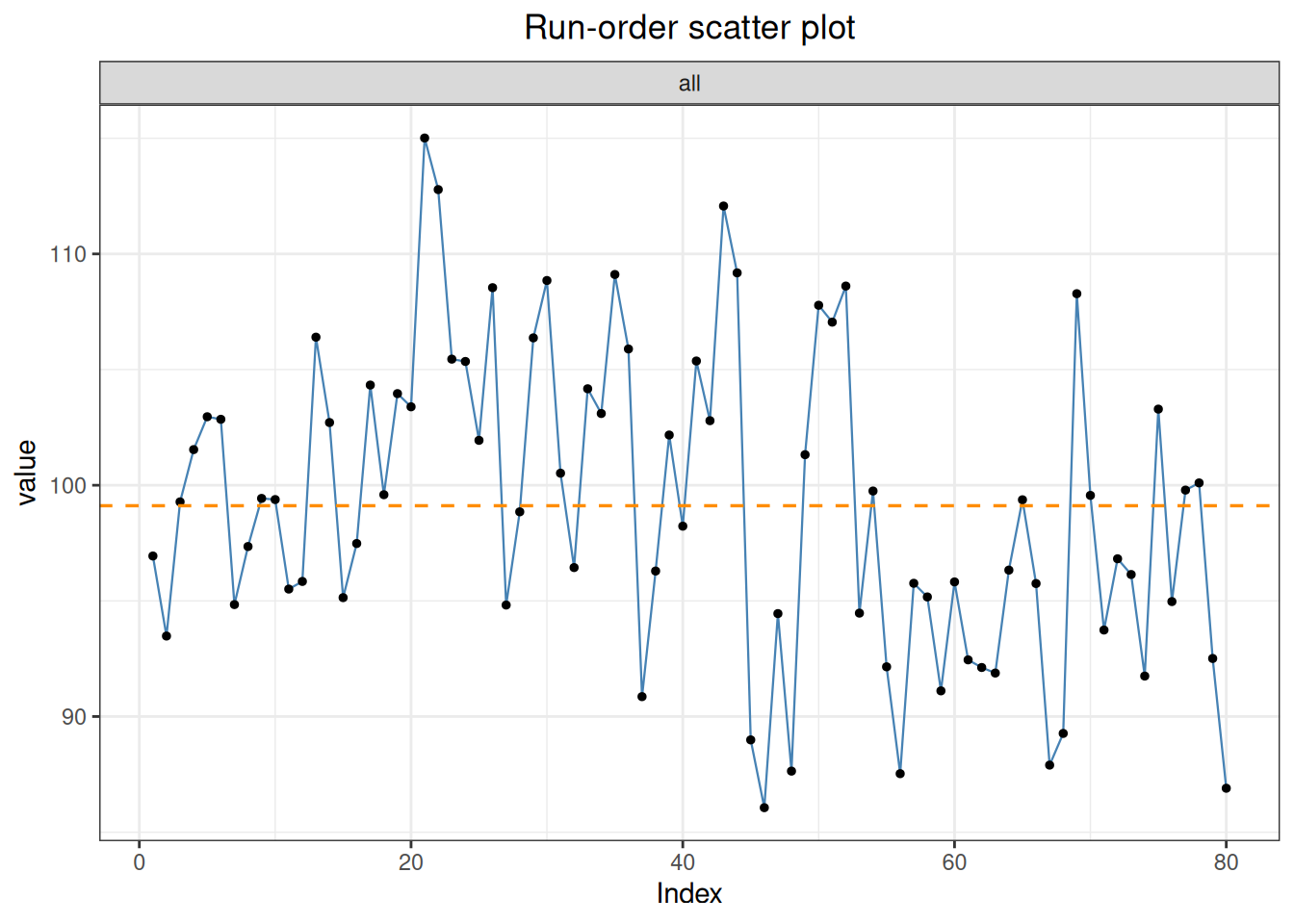

Code

plot(p, type = "qq")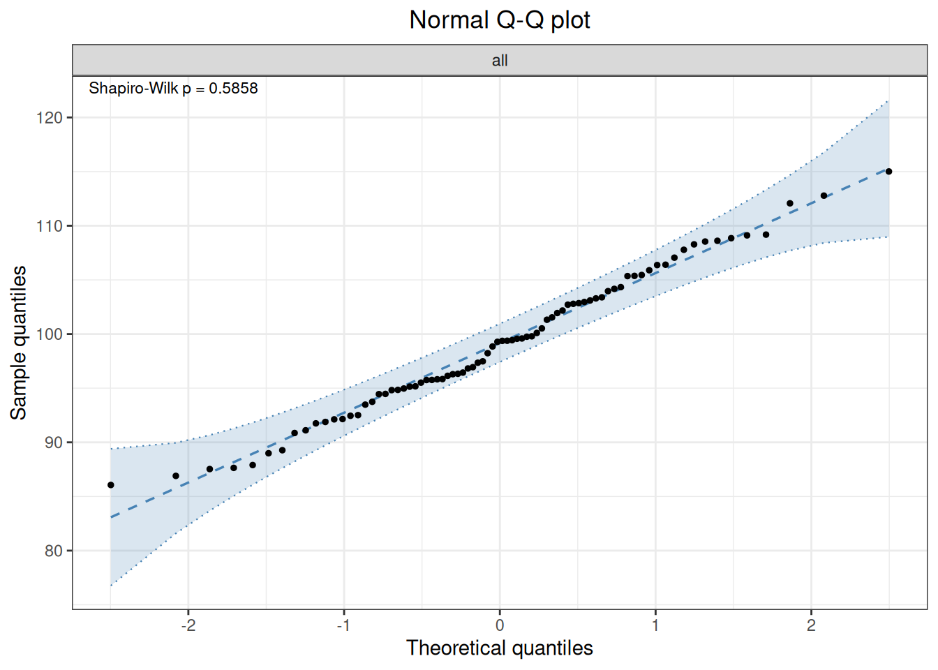

value ~ day/run means day, nested run within day, and replicate residual error. outlier() accepts "grubbs" or "iqr"; normal(method="auto") selects by sample size. NegVC is supplied to variance(), not to precision():

Code

p <- variance(p, NegVC = TRUE)

13.2.2 Multiple Samples and a Sadler Profile

Code

profile_data <- as.data.frame(read_csv(
  "./data/013-精密度分析/precision-profile.csv", show_col_types = FALSE
))
profile_data$sample <- factor(profile_data$sample)
profile_data$day <- factor(profile_data$day)
profile_data$rep <- factor(profile_data$rep)

p2 <- precision(profile_data, value ~ day, by = "sample")
p2 <- variance(p2)

Variance components
 sample component       VC %Total      SD  CV[%] Method
-------------------------------------------------------
     L1       day   0.6376   63.0  0.7985 3.9446  anova
     L1     error   0.3750   37.0  0.6124 3.0250  anova
     L2       day   5.7139   75.1  2.3904 4.7584  anova
     L2     error   1.8937   24.9  1.3761 2.7393  anova
     L3       day   3.3913   15.7  1.8415 1.8088  anova
     L3     error  18.1466   84.3  4.2599 4.1840  anova
     L4       day  30.5549   54.6  5.5276 2.7529  anova
     L4     error  25.4525   45.4  5.0451 2.5126  anova
     L5       day   0.0000    0.0  0.0000 0.0000  anova
     L5     error 171.7986  100.0 13.1072 3.3003  anova

Code

p2 <- ci(p2)

Confidence intervals (SD)
 sample component estimate  lower   upper
-----------------------------------------
     L1     total   1.0063 0.6007  2.9368
     L1       day   0.7985 0.0000  1.4267
     L1     error   0.6124 0.4391  1.0108
     L2     total   2.7582 1.5714  9.9889
     L2       day   2.3904 0.0000  4.2023
     L2     error   1.3761 0.9868  2.2716
     L3     total   4.6409 3.2872  7.8819
     L3       day   1.8415 0.0000  4.1779
     L3     error   4.2599 3.0547  7.0319
     L4     total   7.4838 4.6166 19.1652
     L4       day   5.5276 0.0000 10.0268
     L4     error   5.0451 3.6177  8.3280
     L5     total  13.1072 9.5629 20.8255
     L5       day   0.0000     NA      NA
     L5     error  13.1072 9.3990 21.6365 

Confidence intervals (%CV)
 sample component estimate  lower   upper
-----------------------------------------
     L1     total   4.9710 2.9673 14.5079
     L1       day   3.9446 0.0000  7.0480
     L1     error   3.0250 2.1692  4.9936
     L2     total   5.4905 3.1281 19.8843
     L2       day   4.7584 0.0000  8.3652
     L2     error   2.7393 1.9643  4.5219
     L3     total   4.5583 3.2287  7.7416
     L3       day   1.8088 0.0000  4.1035
     L3     error   4.1840 3.0003  6.9067
     L4     total   3.7271 2.2992  9.5447
     L4       day   2.7529 0.0000  4.9936
     L4     error   2.5126 1.8017  4.1476
     L5     total   3.3003 2.4078  5.2436
     L5       day   0.0000     NA      NA
     L5     error   3.3003 2.3666  5.4478

Code

plot(p2, type = "var")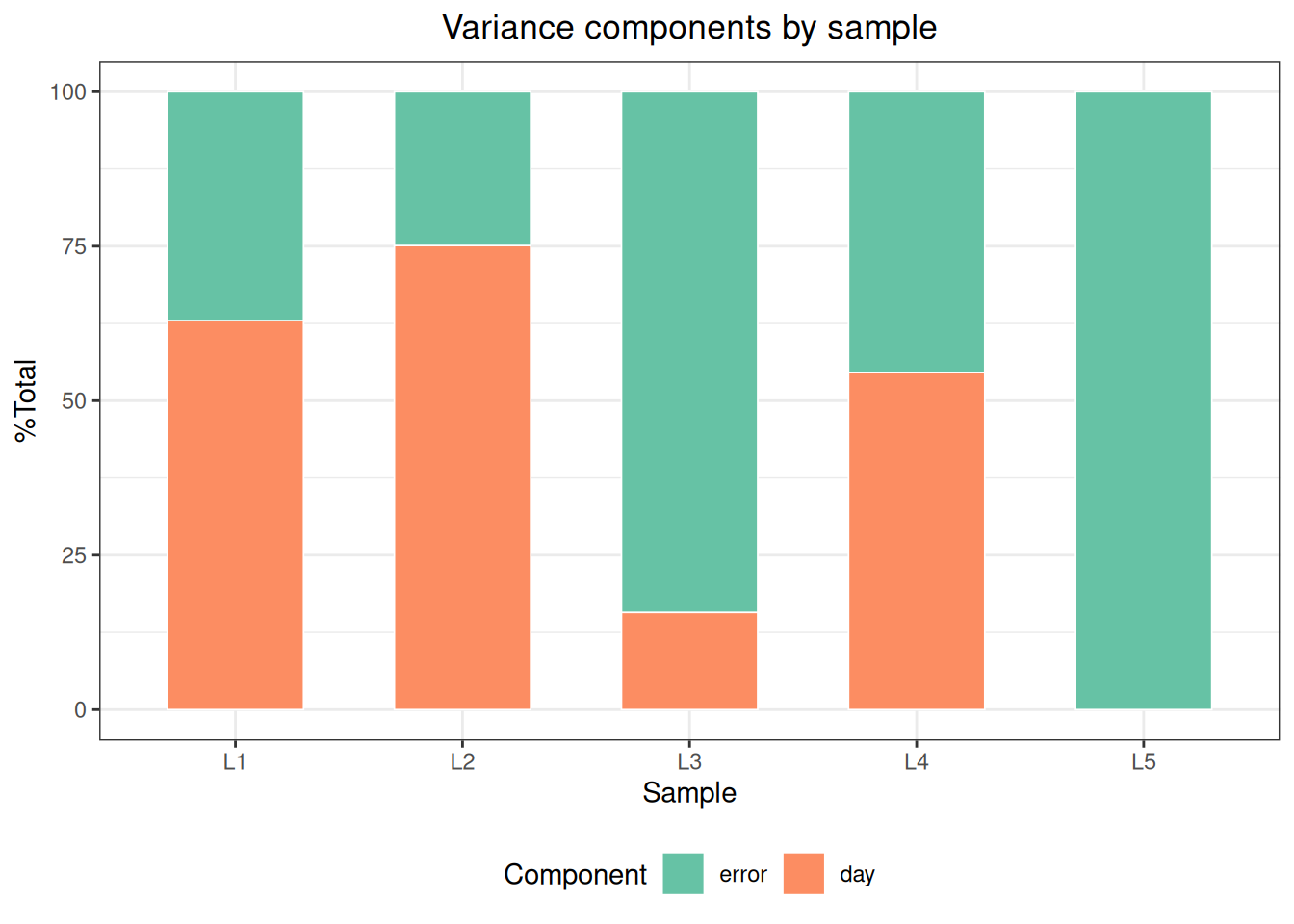

Code

list_sadler()

Sadler Precision Profile Models

   1  Constant variance     sigma^2 = beta1
   2  Constant CV           sigma^2 = beta1 * u^2
   3  Mixed (const + prop var)  sigma^2 = beta1 + beta2 * u^2
   4  Constrained power (const exponent)  sigma^2 = (beta1 + beta2 * u)^2
   5  Alternative constrained power  sigma^2 = beta1 + beta2 * u^K
   6  Unconstrained power (with min)  sigma^2 = beta1 + beta2 * u + beta3 * u^J
   7  Alternative unconstrained power  sigma^2 = beta1 + beta2 * u^J
   8  Unconstrained power (Sadler default)  sigma^2 = (beta1 + beta2 * u)^J
   9  CLSI EP17-like        sigma^2 = beta1 * u^J
  10  CLSI EP17 exact (log-log)  CV = beta1 * u^J

Code

p2 <- profile(p2, model.no = 1:10)

Precision profiles -- Sadler
  total: sigma^2 = 0.0000 + 0.0086 * u^J  (AIC = 56.45, R^2 = 0.9847)
  day: sigma^2 = 0.0000 + 0.0095 * u^J  (AIC = 43.46, R^2 = 0.8919)
  error: sigma^2 = 0.0010 * u^2  (AIC = 55.96, R^2 = 0.9806)

Code

plot(p2, type = "profile")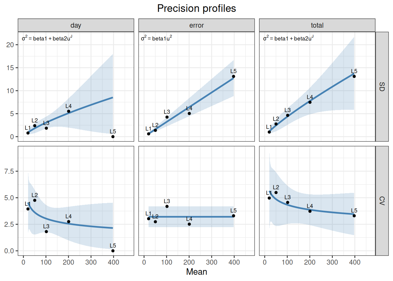

Each variance component needs at least three finite-SD concentrations for profile fitting. The profile can predict SD/CV at arbitrary concentrations for applications such as functional sensitivity, but predictions outside the observed range are extrapolations.

13.2.3 Multicenter Precision

Code

sites_data <- as.data.frame(read_csv(
  "./data/013-精密度分析/precision-sites.csv", show_col_types = FALSE
))
p3 <- precision(sites_data, value ~ site/day/run, by = "sample")
p3 <- variance(p3)

Variance components
 sample    component      VC %Total     SD  CV[%] Method
--------------------------------------------------------
     S1         site  0.2746   10.4 0.5241 1.0550  anova
     S1     site:day  0.0000    0.0 0.0000 0.0000  anova
     S1 site:day:run  0.3553   13.4 0.5960 1.1998  anova
     S1        error  2.0231   76.3 1.4223 2.8632  anova
     S2         site  0.7117    8.6 0.8436 0.8359  anova
     S2     site:day  0.1018    1.2 0.3191 0.3162  anova
     S2 site:day:run  0.9106   11.0 0.9543 0.9456  anova
     S2        error  6.5670   79.2 2.5626 2.5392  anova
     S3         site 22.0901   42.6 4.7000 2.3517  anova
     S3     site:day  2.6252    5.1 1.6202 0.8107  anova
     S3 site:day:run  0.0000    0.0 0.0000 0.0000  anova
     S3        error 27.1915   52.4 5.2145 2.6091  anova

Code

knitr::kable(report(p3, run = "run", day = "day", site = "site"))

Sample Description	Mean Value	Repeatability SD	%CV Repeatability	Reproducibility SD	%CV Reproducibility
S1	49.6766	1.4223	2.8632	1.6288	3.2788
S2	100.9203	2.5626	2.5392	2.8794	2.8532
S3	199.8592	5.2145	2.6091	7.2046	3.6049

To analyze each site separately, use multiple grouping columns while retaining all runs within each subset:

Code

p3s <- precision(sites_data, value ~ day/run, by = c("site", "sample"))
p3s <- variance(p3s)

Variance components
 sample component      VC %Total     SD  CV[%] Method
-----------------------------------------------------
   A.S1       day  0.0000    0.0 0.0000 0.0000  anova
   A.S1   day:run  0.1646    6.8 0.4057 0.8231  anova
   A.S1     error  2.2677   93.2 1.5059 3.0553  anova
   B.S1       day  0.0000    0.0 0.0000 0.0000  anova
   B.S1   day:run  0.5459   23.5 0.7389 1.4758  anova
   B.S1     error  1.7784   76.5 1.3335 2.6637  anova
   A.S2       day  0.3241    4.3 0.5693 0.5602  anova
   A.S2   day:run  0.1523    2.0 0.3903 0.3840  anova
   A.S2     error  7.0483   93.7 2.6549 2.6124  anova
   B.S2       day  0.0000    0.0 0.0000 0.0000  anova
   B.S2   day:run  1.6690   21.5 1.2919 1.2891  anova
   B.S2     error  6.0856   78.5 2.4669 2.4616  anova
   A.S3       day  4.4871   15.6 2.1183 1.0420  anova
   A.S3   day:run  1.7006    5.9 1.3041 0.6415  anova
   A.S3     error 22.5797   78.5 4.7518 2.3375  anova
   B.S3       day  0.7633    2.3 0.8737 0.4448  anova
   B.S3   day:run  0.0000    0.0 0.0000 0.0000  anova
   B.S3     error 31.8033   97.7 5.6394 2.8709  anova

Code

knitr::kable(report(p3s, run = "run", day = "day"))

Sample Description	Mean Value	Repeatability SD	%CV Repeatability	Within-Laboratory Precision SD	%CV Within-Laboratory Precision
A.S1	49.2884	1.5059	3.0553	1.5596	3.1642
B.S1	50.0647	1.3335	2.6637	1.5246	3.0452
A.S2	101.6249	2.6549	2.6124	2.7431	2.6993
B.S2	100.2158	2.4669	2.4616	2.7847	2.7787
A.S3	203.2864	4.7518	2.3375	5.3635	2.6384
B.S3	196.4320	5.6394	2.8709	5.7067	2.9052

13.2.4 More Complex Nested Models

precision() can represent other VCA hierarchies, for example operator, day, and run:

Code

custom_data <- as.data.frame(read_csv(
  "./data/013-精密度分析/precision-custom.csv", show_col_types = FALSE
))
p4 <- precision(custom_data, value ~ operator/day/run)
p4 <- variance(p4)

Variance components
 sample        component     VC %Total     SD  CV[%] Method
-----------------------------------------------------------
    all         operator 2.2914   11.8 1.5137 1.4898  anova
    all     operator:day 6.3159   32.4 2.5132 2.4734  anova
    all operator:day:run 3.2463   16.7 1.8017 1.7733  anova
    all            error 7.6322   39.2 2.7627 2.7190  anova

13.2.5 Standard-Data Cross-Checks

The supplied EP05-A3 Appendix A and B files can be analyzed using the same pattern. Appendix A is a balanced day/run design; Appendix B is a multicenter site/day design with samples grouped by by = "sample":

Code

ep05_a <- as.data.frame(read_csv(
  "./data/013-精密度分析/std-ep05-appendix-a-glucose.csv", show_col_types = FALSE
))
ep05_a$day <- factor(ep05_a$day)
ep05_a$run <- factor(ep05_a$run)
ep05_a_precision <- precision(ep05_a, result ~ day/run)
ep05_a_precision <- variance(ep05_a_precision, NegVC = FALSE)

Variance components
 sample component     VC %Total     SD  CV[%] Method
----------------------------------------------------
    all       day 1.9586   15.1 1.3995 0.5731  anova
    all   day:run 3.0750   23.8 1.7536 0.7181  anova
    all     error 7.9000   61.1 2.8107 1.1510  anova

Code

ep05_a_precision <- ci(ep05_a_precision)

Confidence intervals (SD)
 sample component estimate  lower  upper
----------------------------------------
    all     total   3.5963 3.0696 4.3430
    all       day   1.3995 0.0000 2.4622
    all   day:run   1.7536 0.0000 2.7858
    all     error   2.8107 2.3076 3.5963 

Confidence intervals (%CV)
 sample component estimate  lower  upper
----------------------------------------
    all     total   1.4727 1.2570 1.7785
    all       day   0.5731 0.0000 1.0083
    all   day:run   0.7181 0.0000 1.1408
    all     error   1.1510 0.9450 1.4727

Code

knitr::kable(report(ep05_a_precision, day = "day", run = "run", digits = 6))

Sample Description	Mean Value	Repeatability SD	%CV Repeatability	Within-Laboratory Precision SD	%CV Within-Laboratory Precision
all	244.2	2.810694	1.15098	3.596325	1.472697

Code

ep05_b <- as.data.frame(read_csv(
  "./data/013-精密度分析/std-ep05-appendix-b-ca19-9.csv", show_col_types = FALSE
))
ep05_b_precision <- precision(ep05_b, result ~ site/day, by = "sample")
ep05_b_precision <- variance(ep05_b_precision)

Variance components
 sample component       VC %Total      SD  CV[%] Method
-------------------------------------------------------
     P1      site   0.3843   35.4  0.6199 5.1312  anova
     P1  site:day   0.1778   16.4  0.4216 3.4899  anova
     P1     error   0.5248   48.3  0.7244 5.9963  anova
     P2      site   1.6189   47.9  1.2724 3.0597  anova
     P2  site:day   0.1232    3.6  0.3509 0.8439  anova
     P2     error   1.6348   48.4  1.2786 3.0747  anova
     P5      site  24.9068   29.3  4.9907 1.3165  anova
     P5  site:day   3.1861    3.7  1.7850 0.4709  anova
     P5     error  56.9669   67.0  7.5476 1.9910  anova
     Q3      site   3.1742   60.4  1.7816 3.1959  anova
     Q3  site:day   0.5232   10.0  0.7233 1.2975  anova
     Q3     error   1.5599   29.7  1.2490 2.2404  anova
     Q4      site  30.0735   75.7  5.4839 3.3104  anova
     Q4  site:day   1.8663    4.7  1.3661 0.8247  anova
     Q4     error   7.8128   19.7  2.7951 1.6873  anova
     Q6      site 164.1097   68.1 12.8105 3.0922  anova
     Q6  site:day   3.0208    1.3  1.7380 0.4195  anova
     Q6     error  73.9590   30.7  8.5999 2.0758  anova

Code

ep05_b_precision <- ci(ep05_b_precision)

Confidence intervals (SD)
 sample component estimate  lower   upper
-----------------------------------------
     P1     total   1.0425 0.7415  1.7535
     P1      site   0.6199 0.0000  1.1178
     P1  site:day   0.4216 0.0000  0.6380
     P1     error   0.7244 0.6148  0.8819
     P2     total   1.8376 1.2313  3.5995
     P2      site   1.2724 0.0000  2.2291
     P2  site:day   0.3509 0.0000  0.7084
     P2     error   1.2786 1.0852  1.5566
     P5     total   9.2228 6.9060 13.8849
     P5      site   4.9907 0.0000  8.9156
     P5  site:day   1.7850 0.0000  3.9426
     P5     error   7.5476 6.4058  9.1888
     Q3     total   2.2929 1.4259  5.7003
     Q3      site   1.7816 0.0000  3.1184
     Q3  site:day   0.7233 0.0000  1.0958
     Q3     error   1.2490 1.0600  1.5205
     Q4     total   6.3050 3.6468 21.1983
     Q4      site   5.4839 0.0000  9.5060
     Q4  site:day   1.3661 0.0000  2.1602
     Q4     error   2.7951 2.3723  3.4029
     Q6     total  15.5271 9.3516 43.6651
     Q6      site  12.8105 0.0000 22.1981
     Q6  site:day   1.7380 0.0000  4.2690
     Q6     error   8.5999 7.2989 10.4699 

Confidence intervals (%CV)
 sample component estimate  lower   upper
-----------------------------------------
     P1     total   8.6292 6.1376 14.5139
     P1      site   5.1312 0.0000  9.2524
     P1  site:day   3.4899 0.0000  5.2812
     P1     error   5.9963 5.0891  7.3001
     P2     total   4.4191 2.9611  8.6559
     P2      site   3.0597 0.0000  5.3606
     P2  site:day   0.8439 0.0000  1.7036
     P2     error   3.0747 2.6095  3.7433
     P5     total   2.4329 1.8217  3.6627
     P5      site   1.3165 0.0000  2.3518
     P5  site:day   0.4709 0.0000  1.0400
     P5     error   1.9910 1.6898  2.4239
     Q3     total   4.1130 2.5578 10.2254
     Q3      site   3.1959 0.0000  5.5938
     Q3  site:day   1.2975 0.0000  1.9656
     Q3     error   2.2404 1.9015  2.7276
     Q4     total   3.8061 2.2014 12.7966
     Q4      site   3.3104 0.0000  5.7384
     Q4  site:day   0.8247 0.0000  1.3040
     Q4     error   1.6873 1.4320  2.0542
     Q6     total   3.7479 2.2573 10.5398
     Q6      site   3.0922 0.0000  5.3581
     Q6  site:day   0.4195 0.0000  1.0305
     Q6     error   2.0758 1.7618  2.5272

Code

knitr::kable(report(ep05_b_precision, day = "day", site = "site", table = "detailed"))

Sample Description	Mean Value	N	Repeatability SD	%CV Repeatability	Between-Run SD	%CV Between-Run	Between-Day SD	%CV Between-Day	Between-Site SD	%CV Between-Site	Within-Laboratory Precision SD	%CV Within-Laboratory Precision	Reproducibility SD	%CV Reproducibility
P1	12.0813	75	0.7244	5.9963	NA	NA	0.4216	3.4899	0.6199	5.1312	0.8382	6.9379	1.0425	8.6292
P2	41.5840	75	1.2786	3.0747	NA	NA	0.3509	0.8439	1.2724	3.0597	1.3259	3.1884	1.8376	4.4191
P5	379.0907	75	7.5476	1.9910	NA	NA	1.7850	0.4709	4.9907	1.3165	7.7558	2.0459	9.2228	2.4329
Q3	55.7467	75	1.2490	2.2404	NA	NA	0.7233	1.2975	1.7816	3.1959	1.4433	2.5890	2.2929	4.1130
Q4	165.6560	75	2.7951	1.6873	NA	NA	1.3661	0.8247	5.4839	3.3104	3.1111	1.8781	6.3050	3.8061
Q6	414.2867	75	8.5999	2.0758	NA	NA	1.7380	0.4195	12.8105	3.0922	8.7738	2.1178	15.5271	3.7479

Standard examples can still differ because of exclusion rules, displayed intermediate values, ANOVA versus REML, and the exact degrees-of-freedom convention. Disclose the path used rather than treating similar rounded values as identical algorithms.

13.3 Complete Standard Cases

13.3.1 CLSI EP05-A3 Appendix A: Glucose 20×2×2

Appendix A uses one patient-plasma pool measured in two runs per day on 20 days, with two replicates per run, for 80 glucose results. The data are complete and balanced; the nested structure is day/run, with replicate measurements forming the residual layer.

Code

ep05_a <- as.data.frame(read_csv(
  "./data/013-精密度分析/std-ep05-appendix-a-glucose.csv",
  show_col_types = FALSE
))
ep05_a$day <- factor(ep05_a$day)
ep05_a$run <- factor(ep05_a$run)
ep05_a$replicate <- factor(ep05_a$replicate)

Code

ep05_a_precision <- precision(
  ep05_a, form = result ~ day/run
)
ep05_a_precision <- variance(ep05_a_precision, NegVC = FALSE)

Variance components
 sample component     VC %Total     SD  CV[%] Method
----------------------------------------------------
    all       day 1.9586   15.1 1.3995 0.5731  anova
    all   day:run 3.0750   23.8 1.7536 0.7181  anova
    all     error 7.9000   61.1 2.8107 1.1510  anova

Code

ep05_a_precision <- ci(ep05_a_precision)

Confidence intervals (SD)
 sample component estimate  lower  upper
----------------------------------------
    all     total   3.5963 3.0696 4.3430
    all       day   1.3995 0.0000 2.4622
    all   day:run   1.7536 0.0000 2.7858
    all     error   2.8107 2.3076 3.5963 

Confidence intervals (%CV)
 sample component estimate  lower  upper
----------------------------------------
    all     total   1.4727 1.2570 1.7785
    all       day   0.5731 0.0000 1.0083
    all   day:run   0.7181 0.0000 1.1408
    all     error   1.1510 0.9450 1.4727

Code

knitr::kable(report(
  ep05_a_precision,
  day = "day", run = "run", digits = 6
))

Sample Description	Mean Value	Repeatability SD	%CV Repeatability	Within-Laboratory Precision SD	%CV Within-Laboratory Precision
all	244.2	2.810694	1.15098	3.596325	1.472697

EP05-A3 Appendix A: ivdtools compared with the standard text
Standard location	Statistic	Standard	ivdtools
EP05-A3 Appendix A	mean	244.20	244.2000
EP05-A3 Appendix A	SS_day	415.80	415.8000
EP05-A3 Appendix A	SS_run_day	281.00	281.0000
EP05-A3 Appendix A	SS_error	316.00	316.0000
EP05-A3 Appendix A	MS_day	21.88	21.8842
EP05-A3 Appendix A	MS_run_day	14.05	14.0500
EP05-A3 Appendix A	MS_error	7.90	7.9000
EP05-A3 Appendix A	V_day	1.96	1.9586
EP05-A3 Appendix A	V_run	3.08	3.0750
EP05-A3 Appendix A	V_error	7.90	7.9000
EP05-A3 Appendix A	SD_repeatability	2.81	2.8107
EP05-A3 Appendix A	SD_within_lab	3.60	3.5963
EP05-A3 Appendix A	CV_repeatability	1.20	1.1510
EP05-A3 Appendix A	CV_within_lab	1.50	1.4727

13.3.2 CLSI EP05-A3 Appendix B: CA19-9 Multicenter Study

Appendix B contains three sites, six samples, five days per site, and five replicates per day, for 450 results. The sites use different instruments and operators but the same reagent and calibrator lots. The nested model is site/day, with replicate measurements as the residual layer.

Code

ep05_b <- as.data.frame(read_csv(
  "./data/013-精密度分析/std-ep05-appendix-b-ca19-9.csv",
  show_col_types = FALSE
))
ep05_b$sample <- factor(ep05_b$sample)
ep05_b$site <- factor(ep05_b$site)
ep05_b$day <- factor(ep05_b$day)
ep05_b$replicate <- factor(ep05_b$replicate)

Code

ep05_b_precision <- precision(
  ep05_b, form = result ~ site/day, by = "sample"
)
ep05_b_precision <- variance(ep05_b_precision)

Variance components
 sample component       VC %Total      SD  CV[%] Method
-------------------------------------------------------
     P1      site   0.3843   35.4  0.6199 5.1312  anova
     P1  site:day   0.1778   16.4  0.4216 3.4899  anova
     P1     error   0.5248   48.3  0.7244 5.9963  anova
     P2      site   1.6189   47.9  1.2724 3.0597  anova
     P2  site:day   0.1232    3.6  0.3509 0.8439  anova
     P2     error   1.6348   48.4  1.2786 3.0747  anova
     P5      site  24.9068   29.3  4.9907 1.3165  anova
     P5  site:day   3.1861    3.7  1.7850 0.4709  anova
     P5     error  56.9669   67.0  7.5476 1.9910  anova
     Q3      site   3.1742   60.4  1.7816 3.1959  anova
     Q3  site:day   0.5232   10.0  0.7233 1.2975  anova
     Q3     error   1.5599   29.7  1.2490 2.2404  anova
     Q4      site  30.0735   75.7  5.4839 3.3104  anova
     Q4  site:day   1.8663    4.7  1.3661 0.8247  anova
     Q4     error   7.8128   19.7  2.7951 1.6873  anova
     Q6      site 164.1097   68.1 12.8105 3.0922  anova
     Q6  site:day   3.0208    1.3  1.7380 0.4195  anova
     Q6     error  73.9590   30.7  8.5999 2.0758  anova

Code

ep05_b_precision <- ci(ep05_b_precision)

Confidence intervals (SD)
 sample component estimate  lower   upper
-----------------------------------------
     P1     total   1.0425 0.7415  1.7535
     P1      site   0.6199 0.0000  1.1178
     P1  site:day   0.4216 0.0000  0.6380
     P1     error   0.7244 0.6148  0.8819
     P2     total   1.8376 1.2313  3.5995
     P2      site   1.2724 0.0000  2.2291
     P2  site:day   0.3509 0.0000  0.7084
     P2     error   1.2786 1.0852  1.5566
     P5     total   9.2228 6.9060 13.8849
     P5      site   4.9907 0.0000  8.9156
     P5  site:day   1.7850 0.0000  3.9426
     P5     error   7.5476 6.4058  9.1888
     Q3     total   2.2929 1.4259  5.7003
     Q3      site   1.7816 0.0000  3.1184
     Q3  site:day   0.7233 0.0000  1.0958
     Q3     error   1.2490 1.0600  1.5205
     Q4     total   6.3050 3.6468 21.1983
     Q4      site   5.4839 0.0000  9.5060
     Q4  site:day   1.3661 0.0000  2.1602
     Q4     error   2.7951 2.3723  3.4029
     Q6     total  15.5271 9.3516 43.6651
     Q6      site  12.8105 0.0000 22.1981
     Q6  site:day   1.7380 0.0000  4.2690
     Q6     error   8.5999 7.2989 10.4699 

Confidence intervals (%CV)
 sample component estimate  lower   upper
-----------------------------------------
     P1     total   8.6292 6.1376 14.5139
     P1      site   5.1312 0.0000  9.2524
     P1  site:day   3.4899 0.0000  5.2812
     P1     error   5.9963 5.0891  7.3001
     P2     total   4.4191 2.9611  8.6559
     P2      site   3.0597 0.0000  5.3606
     P2  site:day   0.8439 0.0000  1.7036
     P2     error   3.0747 2.6095  3.7433
     P5     total   2.4329 1.8217  3.6627
     P5      site   1.3165 0.0000  2.3518
     P5  site:day   0.4709 0.0000  1.0400
     P5     error   1.9910 1.6898  2.4239
     Q3     total   4.1130 2.5578 10.2254
     Q3      site   3.1959 0.0000  5.5938
     Q3  site:day   1.2975 0.0000  1.9656
     Q3     error   2.2404 1.9015  2.7276
     Q4     total   3.8061 2.2014 12.7966
     Q4      site   3.3104 0.0000  5.7384
     Q4  site:day   0.8247 0.0000  1.3040
     Q4     error   1.6873 1.4320  2.0542
     Q6     total   3.7479 2.2573 10.5398
     Q6      site   3.0922 0.0000  5.3581
     Q6  site:day   0.4195 0.0000  1.0305
     Q6     error   2.0758 1.7618  2.5272

Code

ep05_b_report <- report(
  ep05_b_precision,
  day = "day", site = "site", table = "detailed", digits = 6
)
ep05_b_report_ci <- report(
  ep05_b_precision,
  day = "day", site = "site", table = "CI", digits = 6
)

EP05-A3 Appendix B: ivdtools compared with the standard text
Standard location	Statistic	Standard	ivdtools
EP05-A3 Appendix B	P1_mean	12.100	12.0813
EP05-A3 Appendix B	P1_SD_R	0.724	0.7244
EP05-A3 Appendix B	P1_SD_WL	0.838	0.8382
EP05-A3 Appendix B	P1_SD_REP	1.040	1.0425
EP05-A3 Appendix B	P1_CV_R	6.000	5.9963
EP05-A3 Appendix B	P1_CV_WL	6.900	6.9379
EP05-A3 Appendix B	P1_CV_REP	8.600	8.6292
EP05-A3 Appendix B	P2_mean	41.600	41.5840
EP05-A3 Appendix B	P2_SD_R	1.280	1.2786
EP05-A3 Appendix B	P2_SD_WL	1.330	1.3259
EP05-A3 Appendix B	P2_SD_REP	1.840	1.8376
EP05-A3 Appendix B	P2_CV_R	3.100	3.0747
EP05-A3 Appendix B	P2_CV_WL	3.200	3.1884
EP05-A3 Appendix B	P2_CV_REP	4.400	4.4191
EP05-A3 Appendix B	P5_mean	379.000	379.0907
EP05-A3 Appendix B	P5_SD_R	7.550	7.5476
EP05-A3 Appendix B	P5_SD_WL	7.760	7.7558
EP05-A3 Appendix B	P5_SD_REP	9.220	9.2228
EP05-A3 Appendix B	P5_CV_R	2.000	1.9910
EP05-A3 Appendix B	P5_CV_WL	2.000	2.0459
EP05-A3 Appendix B	P5_CV_REP	2.400	2.4329
EP05-A3 Appendix B	Q3_mean	55.700	55.7467
EP05-A3 Appendix B	Q3_SD_R	1.250	1.2490
EP05-A3 Appendix B	Q3_SD_WL	1.440	1.4433
EP05-A3 Appendix B	Q3_SD_REP	2.290	2.2929
EP05-A3 Appendix B	Q3_CV_R	2.200	2.2404
EP05-A3 Appendix B	Q3_CV_WL	2.600	2.5890
EP05-A3 Appendix B	Q3_CV_REP	4.100	4.1130
EP05-A3 Appendix B	Q4_mean	166.000	165.6560
EP05-A3 Appendix B	Q4_SD_R	2.800	2.7951
EP05-A3 Appendix B	Q4_SD_WL	3.110	3.1111
EP05-A3 Appendix B	Q4_SD_REP	6.300	6.3050
EP05-A3 Appendix B	Q4_CV_R	1.700	1.6873
EP05-A3 Appendix B	Q4_CV_WL	1.900	1.8781
EP05-A3 Appendix B	Q4_CV_REP	3.800	3.8061
EP05-A3 Appendix B	Q6_mean	414.000	414.2867
EP05-A3 Appendix B	Q6_SD_R	8.600	8.5999
EP05-A3 Appendix B	Q6_SD_WL	8.770	8.7738
EP05-A3 Appendix B	Q6_SD_REP	15.500	15.5271
EP05-A3 Appendix B	Q6_CV_R	2.100	2.0758
EP05-A3 Appendix B	Q6_CV_WL	2.100	2.1178
EP05-A3 Appendix B	Q6_CV_REP	3.700	3.7479

13.3.3 CLSI EP15-A3: Ferritin 5×5 Verification

The complete EP15 case contains three serum ferritin levels, measured for five days with five replicates per day. Keep the raw data intact, then reproduce the standard case’s prespecified Grubbs exclusion of 30.2 µg/L from Level 1, Day 1, Replicate 3. This exclusion reproduces the standard case and is not selected retrospectively by the code.

Code

ep15_ferritin_raw <- as.data.frame(read_csv(
  "./data/013-精密度分析/std-ep15-ferritin.csv", show_col_types = FALSE
))
ep15_ferritin_raw$sample <- factor(ep15_ferritin_raw$sample)
ep15_ferritin_raw$run <- factor(ep15_ferritin_raw$run)
ep15_ferritin_raw$replicate <- factor(ep15_ferritin_raw$replicate)

ep15_exclude <- with(
  ep15_ferritin_raw,
  sample == 1L & run == 1L & replicate == 3L
)
ep15_ferritin_raw[ep15_exclude, ]

  run replicate sample result
7   1         3      1   30.2

Code

# Exclude the prespecified result.
ep15_ferritin <- ep15_ferritin_raw[!ep15_exclude, ]

After exclusion, Level 1 has 24 results, with four replicates on Day 1; Levels 2 and 3 each retain 25 results. Split by sample and fit one result ~ run model for each level. run represents the between-run component, while daily replicates form the residual error component.

Code

# Separate levels to compare ANOVA and REML explicitly.
ep15_ferritin_list <- split(ep15_ferritin, ep15_ferritin$sample)
ep15_level_1 <- droplevels(ep15_ferritin_list[["1"]])
ep15_level_2 <- droplevels(ep15_ferritin_list[["2"]])
ep15_level_3 <- droplevels(ep15_ferritin_list[["3"]])

# Level 1
ep15_level_1_fit <- precision(ep15_level_1, result ~ run)
# The unbalanced design automatically switches to REML.
ep15_level_1_fit_r <- variance(
  ep15_level_1_fit, NegVC = FALSE
)

Variance components
 sample component     VC %Total     SD  CV[%] Method
----------------------------------------------------
    all       run 0.2820   27.5 0.5311 2.0816   reml
    all     error 0.7423   72.5 0.8616 3.3770   reml

Code

# Use ANOVA explicitly to match the standard case.
ep15_level_1_fit <- variance(
  ep15_level_1_fit, method = "anova", NegVC = FALSE
)

Variance components
 sample component     VC %Total     SD  CV[%] Method
----------------------------------------------------
    all       run 0.2804   27.4 0.5295 2.0756  anova
    all     error 0.7414   72.6 0.8610 3.3749  anova

Code

ep15_level_1_fit <- ci(ep15_level_1_fit, digits = 6)

Confidence intervals (SD)
 sample component estimate    lower    upper
--------------------------------------------
    all     total 1.010837 0.752556 1.539604
    all       run 0.529550 0.000000 0.944544
    all     error 0.861028 0.654803 1.257592 

Confidence intervals (%CV)
 sample component estimate    lower    upper
--------------------------------------------
    all     total 3.962125 2.949754 6.034706
    all       run 2.075649 0.000000 3.702279
    all     error 3.374924 2.566597 4.929319

Code

# Level 2
ep15_level_2_fit <- precision(ep15_level_2, result ~ run)
ep15_level_2_fit <- variance(
  ep15_level_2_fit, method = "anova", NegVC = FALSE
)

Variance components
 sample component     VC %Total     SD  CV[%] Method
----------------------------------------------------
    all       run 2.5400   44.6 1.5937 1.1374  anova
    all     error 3.1600   55.4 1.7776 1.2687  anova

Code

ep15_level_2_fit <- ci(ep15_level_2_fit, digits = 6)

Confidence intervals (SD)
 sample component estimate    lower    upper
--------------------------------------------
    all     total 2.387467 1.701094 3.999257
    all       run 1.593738 0.000000 2.636950
    all     error 1.777639 1.359999 2.567034 

Confidence intervals (%CV)
 sample component estimate    lower    upper
--------------------------------------------
    all     total 1.703873 1.214026 2.854166
    all       run 1.137409 0.000000 1.881922
    all     error 1.268655 0.970596 1.832025

Code

# Level 3
ep15_level_3_fit <- precision(ep15_level_3, result ~ run)
ep15_level_3_fit <- variance(
  ep15_level_3_fit, method = "anova", NegVC = FALSE
)

Variance components
 sample component       VC %Total      SD  CV[%] Method
-------------------------------------------------------
    all       run 102.6080   47.5 10.1296 1.6262  anova
    all     error 113.5200   52.5 10.6546 1.7105  anova

Code

ep15_level_3_fit <- ci(ep15_level_3_fit, digits = 6)

Confidence intervals (SD)
 sample component  estimate     lower     upper
-----------------------------------------------
    all     total 14.701292 10.382650 25.141336
    all       run 10.129561  0.000000 16.638736
    all     error 10.654576  8.151381 15.385949 

Confidence intervals (%CV)
 sample component estimate    lower    upper
--------------------------------------------
    all     total 2.360213 1.666878 4.036305
    all       run 1.626246 0.000000 2.671259
    all     error 1.710534 1.308660 2.470130

Extract the total mean, run variance component, repeatability SD, and total within-laboratory SD from each object and compare them with the displayed standard values:

EP15-A3 ferritin: ivdtools compared with the standard text
Sample	Statistic	Standard	ivdtools
Level 1	overall mean	25.5000	25.5125
Level 1	between-run variance	0.2805	0.2804
Level 1	repeatability SD	0.8600	0.8610
Level 1	within-laboratory SD	1.0100	1.0108
Level 2	overall mean	140.1000	140.1200
Level 2	between-run variance	2.5400	2.5400
Level 2	repeatability SD	1.7800	1.7776
Level 2	within-laboratory SD	2.4000	2.3875
Level 3	overall mean	623.0000	622.8800
Level 3	between-run variance	102.6100	102.6080
Level 3	repeatability SD	10.7000	10.6546
Level 3	within-laboratory SD	14.7000	14.7013

The recalculated results for all three levels agree with or are close to the displayed standard values. Level 1 is unbalanced after exclusion, so small differences in variance components arise from unbalanced-data calculation details and intermediate rounding. For Level 2, the exact within-laboratory SD is 2.3875 µg/L, while the standard displays 2.40 µg/L after rounding its variance components. The standard case passes all three levels under its stated PI and UVL criteria; that conclusion applies only to the stated claims and limits.

13.3.4 WS/T 408–2024: Precision Verification

WS/T 408 Appendix A.2 uses two HDL-C levels, five batches per level, and three replicates per batch. After import, verify that each sample and batch contains three results.

Code

wst408_precision <- as.data.frame(read_csv(
  "./data/013-精密度分析/std-wst408-precision.csv",
  show_col_types = FALSE
))
wst408_precision$sample <- factor(wst408_precision$sample)
wst408_precision$batch <- factor(wst408_precision$batch)
wst408_precision$replicate <- factor(wst408_precision$replicate)

Code

wst408_precision_fit <- precision(
  wst408_precision,
  result ~ batch,
  by = "sample"
)
wst408_precision_fit <- variance(
  wst408_precision_fit,
  method = "anova",
  NegVC = FALSE
)

Variance components
 sample component     VC %Total     SD  CV[%] Method
----------------------------------------------------
  样品1     batch 0.0001   10.9 0.0080 0.7637  anova
  样品1     error 0.0005   89.1 0.0228 2.1884  anova
  样品2     batch 0.0001   12.1 0.0091 0.5892  anova
  样品2     error 0.0006   87.9 0.0246 1.5898  anova

Code

wst408_precision_fit <- ci(wst408_precision_fit, digits = 6)

Confidence intervals (SD)
 sample component estimate    lower    upper
--------------------------------------------
  样品1     total 0.024152 0.017523 0.038843
  样品1     batch 0.007958 0.000000 0.020611
  样品1     error 0.022804 0.015933 0.040019
  样品2     total 0.026268 0.019035 0.042360
  样品2     batch 0.009129 0.000000 0.022737
  样品2     error 0.024631 0.017210 0.043225 

Confidence intervals (%CV)
 sample component estimate    lower    upper
--------------------------------------------
  样品1     total 2.317879 1.681694 3.727688
  样品1     batch 0.763745 0.000000 1.978014
  样品1     error 2.188437 1.529098 3.840561
  样品2     total 1.695429 1.228567 2.734049
  样品2     batch 0.589202 0.000000 1.467529
  样品2     error 1.589755 1.110789 2.789914

WS/T 408 Appendix A.2: ivdtools compared with the standard text
Sample	Statistic	Standard	ivdtools
Level 1	overall mean	1.0420	1.0420
Level 1	s_WR	0.0228	0.0228
Level 1	s_WL	0.0242	0.0242
Level 1	CV_WL (%)	NA	2.3179
Level 2	overall mean	1.5493	1.5493
Level 2	s_WR	0.0246	0.0246
Level 2	s_WL	0.0263	0.0263
Level 2	CV_WL (%)	NA	1.6954

13.3.5 YY/T 1789.1–2021 Appendix A: 25-Hydroxyvitamin D

Appendix A provides complete 20-day × 2-run × 2-replicate data, for 80 results.

Code

yyt1789_1 <- read.csv(
  "./data/013-精密度分析/std-yyt1789-1-appendix-a.csv"
)
yyt1789_1$day <- factor(yyt1789_1$day)
yyt1789_1$run <- factor(yyt1789_1$run)

yyt1789_1_fit <- precision(yyt1789_1, result ~ day/run)
yyt1789_1_fit <- variance(
  yyt1789_1_fit, method = "anova"
)

Variance components
 sample component     VC %Total     SD  CV[%] Method
----------------------------------------------------
    all       day 0.1769   36.2 0.4206 2.4324  anova
    all   day:run 0.0648   13.2 0.2545 1.4721  anova
    all     error 0.2475   50.6 0.4975 2.8773  anova

Code

yyt1789_1_fit <- ci(yyt1789_1_fit)

Confidence intervals (SD)
 sample component estimate  lower  upper
----------------------------------------
    all     total   0.6994 0.5861 0.8674
    all       day   0.4206 0.0000 0.5991
    all   day:run   0.2545 0.0000 0.4400
    all     error   0.4975 0.4084 0.6365 

Confidence intervals (%CV)
 sample component estimate  lower  upper
----------------------------------------
    all     total   4.0450 3.3897 5.0170
    all       day   2.4324 0.0000 3.4650
    all   day:run   1.4721 0.0000 2.5448
    all     error   2.8773 2.3623 3.6815

YY/T 1789.1–2021 Appendix A: ivdtools compared with the standard text
Standard location	Statistic	Standard	ivdtools
YY/T 1789.1 Appendix A	mean	17.290	17.2898
YY/T 1789.1 Appendix A	repeatability SD	0.497	0.4975
YY/T 1789.1 Appendix A	within-laboratory SD	0.699	0.6994
YY/T 1789.1 Appendix A	repeatability CV (%)	2.900	2.8773
YY/T 1789.1 Appendix A	within-laboratory CV (%)	4.000	4.0450
YY/T 1789.1 Appendix A	repeatability CI lower	0.408	0.4084
YY/T 1789.1 Appendix A	repeatability CI upper	0.637	0.6365
YY/T 1789.1 Appendix A	within-laboratory CI lower	0.586	0.5861
YY/T 1789.1 Appendix A	within-laboratory CI upper	0.867	0.8674