%%{init: {"theme":"base","themeVariables":{"primaryColor":"#EAF2FB","primaryBorderColor":"#2780E3","primaryTextColor":"#212529","lineColor":"#6C757D","secondaryColor":"#EAF7E6","tertiaryColor":"#FFF4E8","fontSize":"13px"},"flowchart":{"nodeSpacing":18,"rankSpacing":24,"padding":6}}}%%

flowchart LR
    A["Binary reference state<br/>Quantitative marker"] --> B["roc()<br/>Complete cases and direction"]
    B --> C["describe()<br/>Data checks"]
    B --> D["auc()<br/>AUC and interval"]
    D --> E["cutoff()<br/>Candidate thresholds and metrics"]
    E --> F["plot() / summary()<br/>Interpretation and reporting"]

    classDef input fill:#EAF2FB,stroke:#2780E3,color:#212529
    classDef process fill:#EAF7E6,stroke:#3FB618,color:#212529
    classDef output fill:#F4EEFB,stroke:#9954BB,color:#212529
    class A input
    class B,C,D,E process
    class F output
11 ROC Curves and Cutoff Determination
This chapter demonstrates how to use ivdtools to evaluate the ability of a quantitative marker to distinguish a target state and, after confirming the classification direction, inspect candidate cutoffs. An ROC curve describes the trade-off between sensitivity and specificity across thresholds, AUC summarizes the complete empirical ROC, and a cutoff represents a particular decision point. These answer different questions.
ImportantScope of Use
ROC conclusions assume that the reference state is correct, the study population is representative, and the positive class is defined correctly. ivdtools currently provides an empirical ROC, trapezoidal AUC, a Hanley–McNeil standard error for a single curve, and two within-sample cutoff criteria. It does not provide partial AUC, intervals at fixed sensitivity or specificity, paired ROC tests, resampling uncertainty for cutoffs, sample-size design, or external validation.
The function automatically selects the geq or leq direction by comparing marker means in the positive and negative groups; there is no separate direction argument. A formal analysis must verify that the automatic direction agrees with the prespecified clinical meaning. An in-sample “optimal” cutoff is subject to selection bias and cannot be interpreted directly as a validated threshold in an independent population or as a recommended standard cutoff.
The single-marker ROC workflow is:
Code
library(ivdtools)
library(readr)
11.1 Main Functions
| Function | Main purpose | Main result |
|---|---|---|
continuous_to_binary() |
Convert a continuous reference variable to 0/1 using a supplied threshold | Original data and a new <variable>_binary column |
roc() |
Create an ROC object and determine common complete cases and direction | Sample information, reference encoding, marker values, and direction |
describe() |
Describe the raw variables in the object | Numeric summaries and categorical frequencies |
auc() |
Calculate empirical ROC, AUC, standard error, and 95% CI | auc_list and auc_table |
cutoff() |
Calculate diagnostic metrics at candidate thresholds and two optimization criteria | cutoff_table |
plot() |
Plot ROC or cutoff–metric curves | ggplot figure |
summary() |
Summarize analysis slots already run | ROC object summary |
11.1.1 Convert a Continuous Reference Variable with continuous_to_binary()
Code
continuous_to_binary(data, cols, cutoff)| Argument | Description |
|---|---|
data |
Data frame. |
cols |
One or more names of numeric columns to convert. |
cutoff |
A finite numeric value. A length-one value is recycled for all columns; otherwise it must have the same length as cols. |
For variable \(j\), the function applies
\[ B_{ij}=I(X_{ij}\ge c_j). \]
The original columns are retained and <variable>_binary is added. Equality at the cutoff is always assigned to 1; the function does not support a <= direction. Use it only when this binary definition has already been established by the protocol or an external reference. Do not repeatedly search for a reference-variable threshold in the same data to improve ROC performance.
The function returns a data frame with the original columns and the new <variable>_binary columns.
11.1.2 Create an Analysis Object with roc()
Code
roc(data, cols, reference, id = NULL, positive = NULL)| Argument | Description |
|---|---|
data |
Data frame. |
cols |
One or more numeric marker-column names. |
reference |
Name of one reference-state column; it may be numeric 0/1, a two-level factor, or a two-value character vector. |
id |
Optional subject identifier; used only to report repeated IDs and does not deduplicate automatically. |
positive |
Positive level for a factor or character reference. If omitted, the last level after sorting is used. For numeric 0/1, 1 is positive when omitted. |
roc() requires the reference and all cols to be finite and complete. Define
\[ R_i=I(Y_i\text{ is complete})\prod_{j=1}^{p}I(X_{ij}\text{ is finite and complete}), \]
and include only subjects with \(R_i=1\) in the object. Even if auc() is later called for only a subset of cols, the analysis sample remains the common complete-case set determined by all markers when the object was created. Create separate objects if each marker should use its own complete cases.
For marker \(X_j\), the source compares group means:
\[ \bar X_{j,+}\ge\bar X_{j,-}\Rightarrow \widehat Y=I(X_j\ge c)\quad(\texttt{geq}), \]
\[ \bar X_{j,+}<\bar X_{j,-}\Rightarrow \widehat Y=I(X_j\le c)\quad(\texttt{leq}). \]
This is a computational direction, not a validation of clinical direction. An extreme value can affect a group mean and select the wrong direction; inspect col_direction and compare it with the protocol.
Main fields include n, n_pos, n_neg, n_total, cols_values, reference_binary, col_direction, and print, followed by describe, auc_list, auc_table, cutoff_table, and mlr_results as later analyses are added.
The returned object has class roc, stores common complete cases, reference states, marker values, and automatic directions, and is updated by subsequent analyses.
11.1.3 Descriptive Statistics with describe()
The function returns a descriptive-statistics data frame. Numeric columns contain sample size, mean, SD, quantiles, and range; categorical columns contain frequencies and percentages.
Code
describe(x, cols = NULL, digits = 4L)When cols=NULL, the function describes all columns in the original data except an explicitly supplied ID, not only ROC markers. Numeric columns provide \(n\), mean, SD, minimum, quartiles, and maximum; factors, characters, and the reference column provide frequencies and percentages. The current implementation does not summarize marker distributions separately by positive and negative group, so group differences require a separate table or plot.
11.1.4 AUC with auc()
Code
auc(x, cols = NULL)The empirical ROC is calculated at every distinct observed value and at the two \(±\infty\) thresholds, and the AUC is integrated by trapezoids over false-positive rate, \(\mathrm{FPR}=1-\mathrm{Sp}\). Equivalently, it is the rank statistic
\[ \widehat A= \frac{1}{n_+n_-} \sum_{i:Y_i=1}\sum_{j:Y_j=0} \left[I(X_i>X_j)+\frac12I(X_i=X_j)\right], \]
with the order reversed when low values represent the positive class. AUC estimates the probability that a randomly selected positive and negative subject are correctly ordered by the selected direction; it is not the accuracy at a particular cutoff.
The current standard error uses the Hanley–McNeil approximation. Let
\[ Q_1=\frac{\widehat A}{2-\widehat A},\qquad Q_2=\frac{2\widehat A^2}{1+\widehat A}, \]
then
\[ \operatorname{SE}(\widehat A)= \sqrt{\frac{ \widehat A(1-\widehat A) (n_+-1)(Q_1-\widehat A^2) (n_--1)(Q_2-\widehat A^2)} {n_+n_-}}. \]
The 95% CI is \(\hat A\pm1.96\,\operatorname{SE}(\widehat A)\), truncated to \([0,1]\). When AUC is exactly 0 or 1, the current implementation returns NA for the standard error and interval rather than an exact or resampling interval.
The updated roc object stores ROC points, AUC, standard error, and interval for each marker in auc_list, with a summary table in auc_table.
11.1.5 Cutoff Analysis with cutoff()
Code
cutoff(x, cols = NULL)Run auc() first. For the geq direction, predicted positive means \(X_i\ge c\); for leq, it means \(X_i\le c\). At each candidate threshold, calculate
\[ \mathrm{Se}=\frac{TP}{TP+FN},\qquad \mathrm{Sp}=\frac{TN}{TN+FP}, \]
\[ \mathrm{PPV}=\frac{TP}{TP+FP},\qquad \mathrm{NPV}=\frac{TN}{TN+FN},\qquad \mathrm{Accuracy}=\frac{TP+TN}{N}. \]
precision in the table means PPV. The two automatic criteria are the maximum of
\[ J(c)=\mathrm{Se}(c)+\mathrm{Sp}(c)-1 \]
(Youden) and the minimum of
\[ d(c)=\sqrt{[1-\mathrm{Se}(c)]^2+[1-\mathrm{Sp}(c)]^2} \]
(Corner). The candidate set consists of observed values and two infinite endpoints; the endpoints complete the ROC but are not reported as optimal finite cutoffs. If several finite thresholds tie, the source selects the first in its internal order: descending for geq and ascending for leq. Thus the automatic result also has a deterministic tie-breaking rule.
WarningObserved-Value Cutoffs versus Open-Interval Cutoffs
Manual EP24 tables often place a cutoff in the open interval between adjacent observations. ivdtools uses observed values as thresholds and assigns equality to the positive side. A report must therefore state the decision rule, such as “results \(≥9.5\) are positive,” rather than only writing “cutoff 9.5”; open-interval endpoints and implemented thresholds must not be conflated.
The updated roc object stores candidate thresholds, confusion matrices, diagnostic metrics, and the two selection criteria in cutoff_table.
11.1.6 Plotting and Summary with plot() and summary()
Code
plot(x, curves = NULL, cutpoint = NULL,
     type = c("roc", "cutoff"))
summary(x)curves=NULLselects all original markers by default;curves="all"selects all original markers and saved MLR models. A character vector such asc("x1", "combined")can mix both.type="roc"plots sensitivity against \(1-\mathrm{Sp}\). An original marker requiresauc()first.cutpointcan be"Youden","Corner", or"all"and requirescutoff()first; it labels only the selected original marker.type="cutoff"plots sensitivity and specificity against finite thresholds for one original marker. Only one original marker may be specified incurves; MLR model probabilities are not currently supported.summary()summarizes analyses already present in the object; it does not automatically rundescribe(),auc(), orcutoff().
plot() invisibly returns a ggplot object; summary() prints and invisibly returns the input roc object.
11.2 Analysis Examples
11.2.1 Teaching Data: Complete Single-Marker Workflow
Code
roc_dat <- as.data.frame(read_csv(
  "./data/011-ROC曲线与cutoff/roc-example.csv",
  show_col_types = FALSE
))
head(roc_dat, 6)
sid ref x1
1 1 0 7.594080
2 2 0 8.312513
3 3 0 5.885744
4 4 0 5.585100
5 5 0 9.568483
6 6 0 2.364555Code
roc_fit <- roc(
  roc_dat, cols = "x1", reference = "ref", id = "sid"
)
print(roc_fit)
ROC Analysis
  Data class:        data.frame
  Total rows:        100
  Complete cases:    100
  Reference:         ref (binary)
  Reference coding:  binary (0/1)
  Positive / Neg:    50 / 50
  Evaluation cols:   1  (x1)
  Duplicate IDs:     none

Analysis slots:
    [ ] Describe
    [ ] AUC
    [ ] Paired AUC comparison
    [ ] Cutoff
    [ ] MLR
Code
roc_fit <- describe(roc_fit, cols = c("x1", "ref"))
Descriptive Statistics
  Variable               n     Mean       SD      Min       Q1   Median       Q3      Max  NA
  ---------------------------------------------------------------------------
  x1                   100   9.2576   4.4744  -0.3894   5.8224   8.5472  12.9591  18.7295

  ref
  Level                Count  Percent
   --------------------------------------
  0                       50    50.0%
  1                       50    50.0%
Code
roc_fit <- auc(roc_fit)
AUC Table
  Column               AUC          95% CI  Direction
  ------------------------------------------------------------
  x1                0.9420  [0.8940, 0.9900]       geq
The AUC in this example is 0.9420, with a Hanley–McNeil 95% CI of 0.8937–0.9903; the direction is geq. These results describe the apparent discrimination of the current 100 teaching cases.
Code
roc_fit <- cutoff(roc_fit)
Optimal Cutoff Analysis
  Column: x1
    Youden / Corner: cutoff = 8.7617  (sens = 0.9000, spec = 0.9200, Youden = 0.8200)

  Full cutoff table:
        Cutoff      Sens      Spec     TP    FP    TN    FN    Youden
  ----------------------------------------------------------------------
           Inf    0.0000    1.0000      0     0    50    50    0.0000
       18.7295    0.0200    1.0000      1     0    50    49    0.0200
       18.5675    0.0400    1.0000      2     0    50    48    0.0400
       18.2248    0.0600    1.0000      3     0    50    47    0.0600
       17.7837    0.0800    1.0000      4     0    50    46    0.0800
       16.4453    0.1000    1.0000      5     0    50    45    0.1000
       15.8893    0.1200    1.0000      6     0    50    44    0.1200
       15.8087    0.1400    1.0000      7     0    50    43    0.1400
       15.6058    0.1600    1.0000      8     0    50    42    0.1600
       15.5003    0.1800    1.0000      9     0    50    41    0.1800
       15.2855    0.2000    1.0000     10     0    50    40    0.2000
       15.0168    0.2200    1.0000     11     0    50    39    0.2200
       14.8639    0.2400    1.0000     12     0    50    38    0.2400
       14.6980    0.2600    1.0000     13     0    50    37    0.2600
       14.4757    0.2800    1.0000     14     0    50    36    0.2800
       14.4469    0.3000    1.0000     15     0    50    35    0.3000
       14.4042    0.3200    1.0000     16     0    50    34    0.3200
       14.1952    0.3400    1.0000     17     0    50    33    0.3400
       14.1938    0.3600    1.0000     18     0    50    32    0.3600
       13.9382    0.3800    1.0000     19     0    50    31    0.3800
       13.7845    0.4000    1.0000     20     0    50    30    0.4000
       13.3718    0.4200    1.0000     21     0    50    29    0.4200
       13.0699    0.4400    1.0000     22     0    50    28    0.4400
       12.9970    0.4600    1.0000     23     0    50    27    0.4600
       12.9854    0.4800    1.0000     24     0    50    26    0.4800
       12.9659    0.5000    1.0000     25     0    50    25    0.5000
       12.9569    0.5200    1.0000     26     0    50    24    0.5200
       12.7812    0.5400    1.0000     27     0    50    23    0.5400
       12.7534    0.5600    1.0000     28     0    50    22    0.5600
       12.5227    0.5800    1.0000     29     0    50    21    0.5800
       12.3440    0.6000    1.0000     30     0    50    20    0.6000
       12.2962    0.6200    1.0000     31     0    50    19    0.6200
       12.1394    0.6400    1.0000     32     0    50    18    0.6400
       12.1354    0.6600    1.0000     33     0    50    17    0.6600
       12.0393    0.6800    1.0000     34     0    50    16    0.6800
       11.7418    0.6800    0.9800     34     1    49    16    0.6600
       11.6642    0.7000    0.9800     35     1    49    15    0.6800
       11.5082    0.7000    0.9600     35     2    48    15    0.6600
       11.4038    0.7200    0.9600     36     2    48    14    0.6800
       11.2133    0.7400    0.9600     37     2    48    13    0.7000
       11.0696    0.7600    0.9600     38     2    48    12    0.7200
       10.3902    0.7800    0.9600     39     2    48    11    0.7400
       10.1719    0.8000    0.9600     40     2    48    10    0.7600
        9.8836    0.8200    0.9600     41     2    48     9    0.7800
        9.5685    0.8200    0.9400     41     3    47     9    0.7600
        9.3526    0.8400    0.9400     42     3    47     8    0.7800
        9.1944    0.8600    0.9400     43     3    47     7    0.8000
        9.1032    0.8800    0.9400     44     3    47     6    0.8200
        8.8558    0.8800    0.9200     44     4    46     6    0.8000
        8.7617    0.9000    0.9200     45     4    46     5    0.8200
        8.5538    0.9000    0.9000     45     5    45     5    0.8000
        8.5406    0.9000    0.8800     45     6    44     5    0.7800
        8.5296    0.9200    0.8800     46     6    44     4    0.8000
        8.5259    0.9200    0.8600     46     7    43     4    0.7800
        8.3125    0.9200    0.8400     46     8    42     4    0.7600
        8.2985    0.9200    0.8200     46     9    41     4    0.7400
        7.9078    0.9200    0.8000     46    10    40     4    0.7200
        7.8493    0.9200    0.7800     46    11    39     4    0.7000
        7.6187    0.9200    0.7600     46    12    38     4    0.6800
        7.5941    0.9200    0.7400     46    13    37     4    0.6600
        7.5556    0.9200    0.7200     46    14    36     4    0.6400
        7.5150    0.9200    0.7000     46    15    35     4    0.6200
        7.4355    0.9200    0.6800     46    16    34     4    0.6000
        7.1837    0.9200    0.6600     46    17    33     4    0.5800
        6.8235    0.9400    0.6600     47    17    33     3    0.6000
        6.8029    0.9400    0.6400     47    18    32     3    0.5800
        6.7765    0.9400    0.6200     47    19    31     3    0.5600
        6.6770    0.9400    0.6000     47    20    30     3    0.5400
        6.5446    0.9400    0.5800     47    21    29     3    0.5200
        6.5440    0.9600    0.5800     48    21    29     2    0.5400
        6.1603    0.9600    0.5600     48    22    28     2    0.5200
        6.0665    0.9600    0.5400     48    23    27     2    0.5000
        6.0554    0.9600    0.5200     48    24    26     2    0.4800
        6.0361    0.9600    0.5000     48    25    25     2    0.4600
        5.9000    0.9600    0.4800     48    26    24     2    0.4400
        5.8857    0.9600    0.4600     48    27    23     2    0.4200
        5.6326    0.9600    0.4400     48    28    22     2    0.4000
        5.6281    0.9600    0.4200     48    29    21     2    0.3800
        5.5851    0.9600    0.4000     48    30    20     2    0.3600
        5.5802    0.9600    0.3800     48    31    19     2    0.3400
        5.4514    0.9600    0.3600     48    32    18     2    0.3200
        5.3207    0.9600    0.3400     48    33    17     2    0.3000
        5.1582    0.9600    0.3200     48    34    16     2    0.2800
        5.0599    0.9600    0.3000     48    35    15     2    0.2600
        5.0167    0.9600    0.2800     48    36    14     2    0.2400
        4.5654    0.9600    0.2600     48    37    13     2    0.2200
        3.9706    0.9800    0.2600     49    37    13     1    0.2400
        3.9552    0.9800    0.2400     49    38    12     1    0.2200
        3.9103    1.0000    0.2400     50    38    12     0    0.2400
        3.7719    1.0000    0.2200     50    39    11     0    0.2200
        3.5881    1.0000    0.2000     50    40    10     0    0.2000
        3.4583    1.0000    0.1800     50    41     9     0    0.1800
        3.4422    1.0000    0.1600     50    42     8     0    0.1600
        2.9673    1.0000    0.1400     50    43     7     0    0.1400
        2.9111    1.0000    0.1200     50    44     6     0    0.1200
        2.7698    1.0000    0.1000     50    45     5     0    0.1000
        2.5203    1.0000    0.0800     50    46     4     0    0.0800
        2.3646    1.0000    0.0600     50    47     3     0    0.0600
        2.2596    1.0000    0.0400     50    48     2     0    0.0400
        0.4733    1.0000    0.0200     50    49     1     0    0.0200
       -0.3894    1.0000    0.0000     50    50     0     0    0.0000
          -Inf    1.0000    0.0000     50    50     0     0    0.0000
Both criteria select 8.76. Because the direction is geq, this means \(x_1\ge8.76\) is classified as positive. In the current sample, sensitivity is 0.90, specificity is 0.92, and the Youden index is 0.82. PPV and NPV also depend on the positive proportion in the study data and cannot be extrapolated directly to populations with a different prevalence.
Code
plot(roc_fit, cutpoint = "Youden")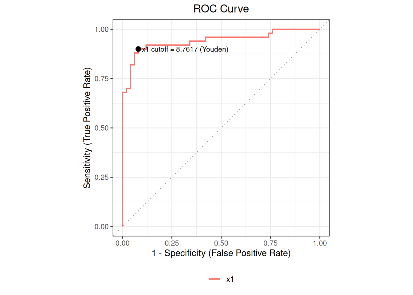
Code
plot(roc_fit, curves = "x1", type = "cutoff", cutpoint = "all")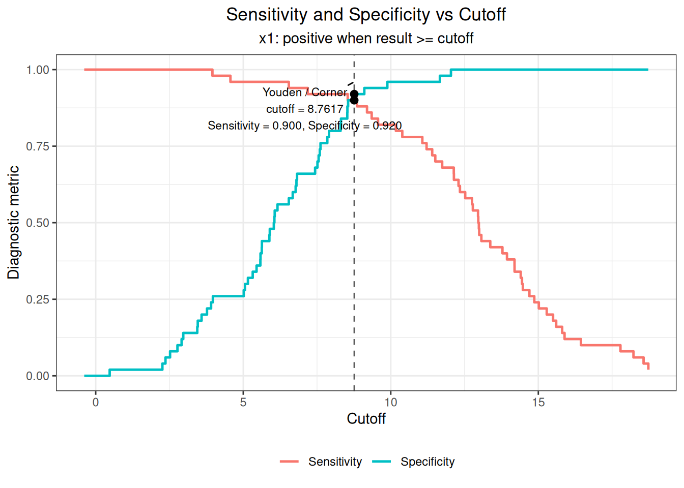
11.2.2 CLSI EP24-A2 Example 1: Empirical ROC and Threshold Intervals
EP24 Table 1 gives 8 subjects and 7 distinct measurement values; there are 4 positive and 4 negative cases, with one cross-group tie at 15.1 ng/mL.
Code
ep24_example1 <- as.data.frame(read_csv(
  "./data/011-ROC曲线与cutoff/std-ep24-example1.csv",
  show_col_types = FALSE
))
ep24_example1_fit <- roc(
  ep24_example1, cols = "assay",
  reference = "status", id = "id"
)
ep24_example1_fit <- auc(ep24_example1_fit)
AUC Table
  Column               AUC          95% CI  Direction
  ------------------------------------------------------------
  assay             0.7812  [0.4390, 1.0000]       geq
Code
ep24_example1_fit <- cutoff(ep24_example1_fit)
Optimal Cutoff Analysis
  Column: assay
    Youden / Corner: cutoff = 9.5000  (sens = 0.7500, spec = 0.7500, Youden = 0.5000)

  Full cutoff table:
        Cutoff      Sens      Spec     TP    FP    TN    FN    Youden
  ----------------------------------------------------------------------
           Inf    0.0000    1.0000      0     0     4     4    0.0000
       24.8000    0.2500    1.0000      1     0     4     3    0.2500
       15.1000    0.5000    0.7500      2     1     3     2    0.2500
        9.5000    0.7500    0.7500      3     1     3     1    0.5000
        7.0000    0.7500    0.5000      3     2     2     1    0.2500
        6.4000    1.0000    0.5000      4     2     2     0    0.5000
        2.1000    1.0000    0.2500      4     3     1     0    0.2500
        1.6000    1.0000    0.0000      4     4     0     0    0.0000
-Inf 1.0000 0.0000 4 4 0 0 0.0000| Standard position | Statistic | Standard result | ivdtools result |
|---|---|---|---|
| EP24-A2 Example 1 | AUC | 0.78 | 0.7812 |
| EP24-A2 Example 1 | Youden cutoff | NA | 9.5000 |
| EP24-A2 Example 1 | Sensitivity | 0.75 | 0.7500 |
| EP24-A2 Example 1 | Specificity | 0.75 | 0.7500 |
EP24 Table 2 places the decision point between adjacent observations, whereas ivdtools uses the observed value 9.5 with a “\(≥\)” rule. This is a difference in threshold notation.
The Youden index also reaches the same maximum across 2.1–6.4. EP24 uses this example to show that the maximum sum and the closest point to the upper-left corner can yield two cutoffs. When Youden values tie, the current software takes 9.5 first under the descending geq candidate order and labels that row Youden / Corner. This is a difference in threshold representation and tie handling, not an error in sensitivity, specificity, or AUC.
11.2.3 CLSI EP24-A2 Appendix D: Single-Curve OxLDL AUC
Appendix D contains 50 subjects, including 28 diagnostic positives and 22 negatives. This section checks only the published OxLDL single-curve AUC, Hanley–McNeil standard error, and normal-approximation interval.
Code
ep24 <- as.data.frame(read_csv(
  "./data/公共/std-ep24-appendix-d.csv",
  show_col_types = FALSE
))
ep24_oxldl <- roc(
  ep24, cols = "oxldl",
  reference = "diagnosis", id = "id"
)
ep24_oxldl <- auc(ep24_oxldl)
AUC Table
  Column               AUC          95% CI  Direction
  ------------------------------------------------------------
oxldl 0.7995 [0.6777, 0.9213] geq| Standard position | Statistic | Standard result | ivdtools result |
|---|---|---|---|
| OxLDL | AUC | 0.800 | 0.799513 |
| OxLDL | SE | 0.062 | 0.062140 |
| OxLDL | CI_lower | 0.680 | 0.677718 |
| OxLDL | CI_upper | 0.920 | 0.921308 |
Appendix D does not recommend an OxLDL cutoff. The following automatically selected result is therefore only a teaching-derived result for the current data:
Code
ep24_oxldl <- cutoff(ep24_oxldl)
Optimal Cutoff Analysis
  Column: oxldl
    Youden / Corner: cutoff = 71.0000  (sens = 0.6429, spec = 0.8636, Youden = 0.5065)

  Full cutoff table:
        Cutoff      Sens      Spec     TP    FP    TN    FN    Youden
  ----------------------------------------------------------------------
           Inf    0.0000    1.0000      0     0    22    28    0.0000
      143.0000    0.0357    1.0000      1     0    22    27    0.0357
      116.0000    0.0714    1.0000      2     0    22    26    0.0714
       96.0000    0.1071    1.0000      3     0    22    25    0.1071
       95.0000    0.1429    1.0000      4     0    22    24    0.1429
       88.0000    0.1786    1.0000      5     0    22    23    0.1786
       86.0000    0.2143    1.0000      6     0    22    22    0.2143
       83.0000    0.2500    1.0000      7     0    22    21    0.2500
       82.0000    0.2857    1.0000      8     0    22    20    0.2857
       78.0000    0.3571    1.0000     10     0    22    18    0.3571
       77.0000    0.4286    0.9545     12     1    21    16    0.3831
       76.0000    0.5357    0.9545     15     1    21    13    0.4903
       74.0000    0.5357    0.9091     15     2    20    13    0.4448
       73.0000    0.5714    0.8636     16     3    19    12    0.4351
       72.0000    0.6071    0.8636     17     3    19    11    0.4708
       71.0000    0.6429    0.8636     18     3    19    10    0.5065
       70.0000    0.6429    0.8182     18     4    18    10    0.4610
       66.0000    0.7143    0.7273     20     6    16     8    0.4416
       64.0000    0.7500    0.6818     21     7    15     7    0.4318
       63.0000    0.7500    0.6364     21     8    14     7    0.3864
       62.0000    0.7500    0.5909     21     9    13     7    0.3409
       61.0000    0.7500    0.5455     21    10    12     7    0.2955
       60.0000    0.8571    0.5000     24    11    11     4    0.3571
       59.0000    0.8571    0.4545     24    12    10     4    0.3117
       57.0000    0.8929    0.4545     25    12    10     3    0.3474
       54.0000    0.8929    0.3636     25    14     8     3    0.2565
       53.0000    0.9286    0.3636     26    14     8     2    0.2922
       52.0000    0.9286    0.3182     26    15     7     2    0.2468
       51.0000    0.9286    0.2727     26    16     6     2    0.2013
       48.0000    0.9286    0.2273     26    17     5     2    0.1558
       45.0000    0.9643    0.2273     27    17     5     1    0.1916
       44.0000    0.9643    0.1818     27    18     4     1    0.1461
       42.0000    0.9643    0.0909     27    20     2     1    0.0552
       41.0000    1.0000    0.0909     28    20     2     0    0.0909
       37.0000    1.0000    0.0455     28    21     1     0    0.0455
       22.0000    1.0000    0.0000     28    22     0     0    0.0000
          -Inf    1.0000    0.0000     28    22     0     0    0.0000