9 Method Comparison and Reference-Material Bias

Method comparison evaluates agreement between candidate and reference procedures on the same samples, corresponding to CLSI EP09. Reference-material bias asks a related but distinct question: how far are repeated measurements of a reference material from its assigned value, including uncertainty in the assigned value?

Analysis path	Main input	Main result
Patient-sample method comparison	Sample ID, comparison and candidate results, optional weights	Difference, regression, agreement limits, outliers, bias at specified levels
Reference-material bias	Replicates, assigned value, and assigned-value uncertainty	Mean, bias, relative bias, and bias interval

Scope of Use

Correlation is not agreement, and a statistically significant bias is not automatically clinically important. Choose the regression and error model before seeing results, preserve the candidate-minus-reference direction, and compare bias and agreement limits with prespecified allowable limits at relevant decision levels.

Code

library(ivdtools)
library(readr)

9.1 Detailed Function Reference

9.1.1 Workflow and Function Overview

Function	Purpose	Return value
replicate_to_mean()	Summarize one or more response columns by sample with mean, SD, and n	Summary data frame
split_by_cutpoints()	Split analysis data at prespecified numeric boundaries	Named data-frame list
mcr()	Create a method-comparison object	mcr object
describe()	Add descriptive statistics	Updated mcr object
correlation()	Add correlation analysis	Updated mcr object
regression()	Fit OLS, WLS, Deming, weighted Deming, or Passing–Bablok regression	Updated mcr object
bland_altman()	Estimate center difference, center interval, and limits of agreement	Updated mcr object
outlier()	Test paired-difference outliers	Updated mcr object
bias()	Calculate bias at specified levels	Updated mcr object
predict()	Forward or inverse prediction	Prediction data frame
reference_bias()	Analyze reference-material bias and intervals	reference_bias object
plot()	Plot scatter, regression, agreement, or bias	ggplot object
summary()	Summarize completed analyses	Original mcr object, invisibly

9.1.2 Summarizing Replicates with replicate_to_mean()

Code

replicate_to_mean(data, x, y, weights = NULL, na.rm = TRUE)

summary_data <- replicate_to_mean(
  raw_data, "sample", c("candidate", "reference")
)

x is the sample-ID column and y can contain one or more numeric result columns. With one column, the function returns x, y_mean, y_sd, and y_n to preserve the original interface. With multiple columns it returns one set of mean, SD, and n columns per variable. The multiple-column mode does not create one common weight because each method has its own precision information.

9.1.3 Splitting Data at Prespecified Cutpoints

Segmentation is data preparation and is not stored in an mcr object. One mcr object always represents one defined data set, so descriptive statistics, correlation, outlier testing, regression, Bland–Altman analysis, bias, and plots use the same sample range.

Code

mcr_data_list <- split_by_cutpoints(
  method_data,
  variable = "reference",
  cutpoints = c(100, 500)
)

mcr_data_list

The console summary has the following form:

Data split by cutpoints
  Variable: reference
  Cutpoints: 100, 500

  segment_1  [-Inf, 100)          n = 35
  segment_2  [100, 500)           n = 62
  segment_3  [500, Inf)           n = 28

The return value is a named data-frame list; each segment retains all original columns and row order:

Code

mcr_data_list$segment_1
mcr_data_list$segment_2
mcr_data_list$segment_3

Use lapply() to create comparison objects for each segment and then run the complete workflow:

Code

mcr_results <- lapply(
  mcr_data_list,
  function(d) mcr(
    d,
    id = "sample",
    candidate = "candidate",
    reference = "reference"
  )
)

mcr_results$segment_1 |>
  describe() |>
  correlation() |>
  regression(method = "deming") |>
  bland_altman()

cutpoints must be finite, strictly increasing, and unique. Intervals are left-closed and right-open, so a cutpoint belongs to the next segment. Empty segments are retained by default to reveal prespecified ranges with no observations; drop_empty = TRUE removes them. Nonfinite segmentation values error by default; na_action = “drop” excludes them and records the count. labels can provide unique list names.

9.1.4 Creating an mcr Object with mcr()

Code

mcr(
  data,
  id,
  candidate,
  reference,
  weights = NULL,
  candidate_sd = NULL,
  reference_sd = NULL,
  candidate_n = NULL,
  reference_n = NULL
)

data must contain one pair of sample-level means per row; duplicate IDs error. id is the sample-ID column. candidate is the evaluated procedure, the regression Y axis, and the first term in the difference. reference is the comparison procedure, the regression X axis, and the second term. weights is an optional finite nonnegative weight column. candidate_sd and reference_sd are optional within-sample SD columns and must be supplied together for lambda = “replicates”. candidate_n and reference_n are optional replicate-count columns and must also be supplied together; if omitted, equal replicate counts are assumed.

The returned mcr object preserves the input data and column names, complete paired values, the input row numbers in complete_idx, and the number of complete pairs n. Later results are stored in describe, correlation, regression, outlier, bland_altman, and bias slots. Split first with split_by_cutpoints() when separate ranges are required.

9.1.5 Descriptive Statistics with describe()

Code

describe(x, cols = NULL, digits = 4L)

x is an mcr object. cols selects additional columns; when omitted, all columns other than ID and the two measurement columns are used, and a minus-prefixed name can exclude a column. digits controls display precision.

The returned object contains complete-pair count, duplicate-ID information, summaries of additional columns, and descriptive statistics for the candidate, reference, and paired difference.

9.1.6 Correlation with correlation()

Code

correlation(
  x,
  method = c("pearson", "spearman", "kendall")
)

method selects Pearson, Spearman, or Kendall. The correlation slot contains coefficient, test statistic, degrees of freedom, P value, interval, and n. Correlation describes common variation and is not agreement.

9.1.7 Regression with regression()

Code

regression(
  x,
  method = c("ols", "wls", "deming", "wdeming", "pb"),
  conf.level = 0.95,
  lambda = 1,
  weights = NULL,
  variance_models = NULL,
  profile_components = c(reference = "total", candidate = "total"),
  ci_method = c(
    "auto", "analytic", "jackknife", "rank",
    "bootstrap_percentile", "bootstrap_standard"
  ),
  bootstrap_replicates = 5000L,
  seed = NULL,
  mdl = NULL,
  weight_iterations = 4L,
  epsilon = NULL
)

method selects ols, wls, deming, wdeming, or pb. conf.level is the regression-parameter confidence level. lambda is candidate-Y variance divided by reference-X variance, as a positive number or “replicates”; the latter uses SD and n supplied to mcr(). weights supports fixed weights, residual, constant_cv, and precision_profile. For precision_profile, variance_models is a list with reference and candidate functions or precision objects that have already been profiled, and profile_components selects the component on each side.

ci_method = “auto” uses analytic intervals for OLS/WLS, complete-refit jackknife for Deming variants, and rank intervals for Passing–Bablok. The explicit bootstrap methods are the K2 percentile and standard methods. At least 5,000 bootstrap replicates are required. seed controls reproducibility without changing the caller’s random-number state. mdl supplies medical decision levels; when bootstrap is run during regression, bias draws for those levels are retained. weight_iterations controls residual-weight updates, and epsilon controls convergence in iterative weighted Deming.

The returned regression slot stores method, intercept, slope, SEs, parameter intervals, intercept–slope covariance, residuals, regression SE, n, input row numbers, confidence level, and, when applicable, R-squared, variance ratio, and weight specification. Iterative weighted Deming also stores convergence, latent concentrations, and final weights. Bootstrap stores the seed, requested/valid/failed counts, and parameter draws. Passing–Bablok follows EP09c Appendix I Algorithm I for vertical pairs, slope -1, and K shifts.

9.1.8 Bland–Altman Analysis with bland_altman()

Code

bland_altman(
  x,
  type = c("difference", "ratio", "percent"),
  x_axis = c("mean", "candidate", "reference"),
  percent_denominator = c("reference", "mean", "candidate"),
  agree.level = 0.95,
  conf.level = 0.95,
  method = c("parametric", "nonparametric", "hodges_lehmann"),
  median_ci_method = c("order_statistic", "interpolated"),
  bootstrap_replicates = 5000L,
  seed = NULL
)

type selects absolute difference, ratio, or percentage difference. x_axis uses the two-method mean, candidate, or reference as horizontal coordinate. percent_denominator independently selects reference, mean, or candidate. agree.level is the LoA coverage proportion, while conf.level is confidence in the center and LoA intervals. The parametric method uses the mean difference, nonparametric uses the ordinary median, and hodges_lehmann uses the HL pseudomedian. median_ci_method selects the conservative order-statistic interval or Appendix F continuous-rank interpolation. bootstrap_replicates and seed control nonparametric LoA resampling.

The bland_altman slot contains center value, center_estimand, center_ci, method-specific center interval, SD, LoA and their intervals, percent denominator, source row numbers, plotting coordinate, and labels. Order-statistic intervals record actual coverage; interpolated intervals record continuous rank and nominal coverage.

9.1.9 Outlier Testing with outlier()

Code

outlier(
  x,
  method = c("grubbs", "esd", "dixon", "iqr"),
  type = c("difference", "percent"),
  percent_denominator = c("reference", "mean", "candidate"),
  alpha = 0.05,
  coef = 1.5,
  ...
)

method selects Grubbs, generalized ESD, Dixon, or IQR. type tests absolute or percent differences, and percent_denominator uses the same definition as bland_altman(). alpha controls the Grubbs, ESD, or Dixon tests; coef controls IQR fences. Additional arguments are passed to the selected test, including r for the maximum number of generalized-ESD candidates.

The returned outlier slot stores method, difference scale, number of outliers, input row numbers, values, test statistics, and critical values. Detection does not authorize deletion.

9.1.10 Bias at Specified Levels with bias()

Code

bias(
  x,
  mdl,
  level = 0.95,
  interval = c("", "confidence", "prediction", "both"),
  ci_method = c("auto", "analytic", "jackknife", "rank",
                "bootstrap_percentile", "bootstrap_standard"),
  bootstrap_replicates = 5000L,
  seed = NULL
)

x must be an mcr object with regression completed. mdl contains one or more reference-scale levels. interval selects confidence, prediction, or both; level is the bias-interval confidence level. ci_method, bootstrap_replicates, and seed control parameter uncertainty. Passing–Bablok under auto uses percentile bootstrap, not jackknife.

The returned bias slot defines bias as fitted candidate minus mdl. After prespecified data segmentation, mdl should lie within that segment to avoid accidental extrapolation.

9.1.11 Prediction with predict()

Code

predict(
  object,
  newdata = NULL,
  reference = NULL,
  candidate = NULL,
  inverse = FALSE,
  interval = c("none", "confidence", "prediction", "both"),
  conf.level = 0.95,
  ci_method = c("auto", "analytic", "jackknife", "rank",
                "bootstrap_percentile", "bootstrap_standard"),
  bootstrap_replicates = 5000L,
  seed = NULL
)

With inverse = FALSE, predict candidate from reference; with inverse = TRUE, algebraically solve for reference from candidate. newdata supplies new values; otherwise the original reference or candidate column is used. The function returns input, predicted value, and requested intervals. Prediction intervals are an ivdtools extension and do not represent EP09c parameter intervals. Inverse prediction is an algebraic back-calculation and does not return an interval.

9.1.12 Reference-Material Bias with reference_bias()

Code

reference_bias(
  data,
  result,
  reference,
  reference_uncertainty,
  level = NULL,
  k = 2
)

data is long-format replicate data. result is the measurement column. reference is a single assigned value, a vector with one value per level, or a column. reference_uncertainty follows the same rules. level optionally identifies material/concentration strata; assignment and uncertainty must be constant within each stratum. k expands the standard uncertainty of the measurement mean into an interval component and defaults to 2.

The returned reference_bias object contains, for each level, total and valid counts, excluded count, mean, SD, standard and expanded uncertainty of the mean, assigned value and its uncertainty, absolute and relative bias, half-width, and interval limits. It also records the input columns, k, and counts.

9.1.13 Plotting and Summary

Code

plot(
  x,
  type = c("scatter", "regression", "bland_altman", "bias"),
  interval = c("none", "confidence", "prediction", "both"),
  conf.level = NULL,
  mdl = NULL
)

type selects scatter, regression, Bland–Altman, or bias plots. interval and conf.level control regression/bias bands; mdl marks medical decision levels. The function invisibly returns a ggplot object. Plots use the same data range as their corresponding analysis slots.

Code

summary(object)

summary prints analyses already completed in the mcr object, does not run missing steps, and invisibly returns the original object.

9.2 Main Functions

Function	Purpose	Return value
`replicate_to_mean()`	Summarize one or more response columns by sample	Summary data frame
`split_by_cutpoints()`	Split data at prespecified numerical boundaries	Named data-frame list
`mcr()`	Create a method-comparison object	`mcr` object
`describe()`	Add descriptive statistics	Updated object
`correlation()`	Add Pearson, Spearman, or Kendall correlation	Updated object
`regression()`	Fit OLS, WLS, Deming, weighted Deming, or Passing–Bablok	Updated object
`bland_altman()`	Estimate center difference and limits of agreement	Updated object
`outlier()`	Test paired-difference outliers	Updated object
`bias()`	Estimate bias at medical decision levels	Updated object
`predict()`	Forward or inverse prediction	Prediction data frame
`reference_bias()`	Analyze reference-material bias and intervals	`reference_bias` object
`plot()` / `summary()`	Plot and summarize completed analyses	Figure or updated object

9.2.1 Summarize Replicates and Split by Cutpoints

Code

replicate_to_mean(data, x = "sample", y = c("candidate", "reference"))
split_by_cutpoints(data, col = "reference", cutpoints = c(30, 80, 150))

The resulting data frame should contain one row per sample and one paired mean for each method. Define cutpoints before analysis and do not repeatedly split to find favorable results.

9.2.2 Build a Method-Comparison Object

Code

mcr(data, id, candidate, reference, weights = NULL,
    candidate_sd = NULL, reference_sd = NULL,
    candidate_n = NULL, reference_n = NULL)

Each row must be one sample-level pair; duplicate IDs are errors. The candidate is the regression Y axis and the first term in candidate-minus-reference differences; the reference is the X axis. Sample-level SD and replicate count columns can support lambda="replicates".

9.2.3 Regression Choices

Code

regression(
  x, method = c("ols", "wls", "deming", "wdeming", "pb"),
  conf.level = 0.95, lambda = 1,
  weights = NULL, variance_models = NULL,
  profile_components = c("total"), ci_method = "auto",
  bootstrap_replicates = 5000, seed = NULL, mdl = NULL
)

OLS treats X error as negligible; Deming accounts for error in both methods; WLS and weighted Deming address concentration-dependent variance; Passing–Bablok uses rank-based slopes without a normal-error model. lambda is the candidate/reference variance ratio and should come from independent precision evidence, not be tuned to match a desired slope. ci_method="auto" uses analytic intervals for OLS/WLS, jackknife for Deming variants, and rank intervals for Passing–Bablok.

9.2.4 Bland–Altman, Outliers, Bias, and Prediction

Code

bland_altman(x, type = c("difference", "ratio", "percent"),
             x_axis = c("mean", "candidate", "reference"))
outlier(x, method = c("grubbs", "esd", "dixon", "iqr"), type = "difference")
bias(x, mdl = c(30, 80, 150), interval = "both")
predict(x, candidate = c(40, 100))
predict(x, reference = c(50, 120), inverse = TRUE)

The Bland–Altman center and limits of agreement describe individual differences, not a test of equality of means. Investigate candidate outliers in the original records and report sensitivity analyses; detection does not authorize automatic deletion.

9.2.5 Reference-Material Bias

Code

reference_bias(
  data,
  result,
  reference,
  reference_uncertainty,
  level = NULL,
  k = 2
)

The function combines the expanded uncertainty of the measured mean with the reference-material uncertainty. It reports results only; state the bias direction and the coverage factor before interpreting the interval.

9.3 Analysis Example

Code

mc_dat <- as.data.frame(read_csv(
  "./data/009-方法学比较与参考物偏倚/method-comparison.csv",
  show_col_types = FALSE
))
mc <- mcr(mc_dat, id = "id", candidate = "candidate", reference = "reference")
mc <- describe(mc)


Descriptive Statistics
  Variable               n     Mean       SD      Min       Q1   Median       Q3      Max  NA
  --------------------------------------------------------------------------- 
    reference (X)       40 105.0000  56.9555  10.0000  57.4750 105.0000 152.5250 200.0000  
    candidate (Y)       40 112.4977  59.2513  11.5900  63.1075 112.5750 159.5925 209.9000  
    Diff (Y-X)          40   7.4977   3.9583   1.2000   5.2725   6.6100   9.7950  22.1000  

  batch
  Level                Count  Percent
   -------------------------------------- 
  B1                      20    50.0%
  B2                      20    50.0%

  sample_type
  Level                Count  Percent
   -------------------------------------- 
  plasma                  13    32.5%
  serum                   14    35.0%
  urine                   13    32.5%

Code

mc <- correlation(mc, method = "pearson")


Correlation
  Method: pearson
  r = 0.9985, 95% CI [0.9971, 0.9992]
  p-value: < 2.2e-16
  n = 40

Code

mc <- regression(mc, method = "deming")


Regression
  Method: Deming
  CI method: jackknife
  Intercept = 3.2588  (SE = 1.4495)
  Slope     = 1.0404  (SE = 0.0100)
  Intercept 95% CI: [0.3245, 6.1930]
  Slope     95% CI: [1.0202, 1.0606]
    H0: slope = 1 -> t = 4.0474, p = 0.0002453
    slope significantly different from 1 (CI excludes 1)
  Sigma     = 3.3319
  n = 40

Code

mc <- bland_altman(mc, type = "difference")


Bland-Altman
  Type:        difference
  Y-axis:      candidate - reference
  X-axis:      Mean of candidate and reference
  Method:       parametric
  n = 40

  Mean diff:       7.4977
  95% CI for mean diff: [6.2318, 8.7637]
  SD diff:         3.9583
  95% LoA: [-0.2603, 15.2558]

  95% CI for LoA:
    Lower LoA: [-2.4419, 1.9213]
    Upper LoA: [13.0742, 17.4374]

Code

mc <- outlier(mc, method = "grubbs", type = "difference")


Outlier
  Method: grubbs
  Data:   Difference (candidate - reference)
  Alpha:  0.05

  1 outlier(s) found:
  Row                Value   Statistic  Critical
   -------------------------------------------------- 
  7                22.1000      3.6891  3.0361

Code

mc <- bias(mc, mdl = c(30, 80, 150), interval = "both")


Bias
  Method: Deming
  Interval: both (95%)
  MDL points: 3
  Bias range: [4.4699, 9.3145]

 mdl     bias ci_lower  ci_upper   pi_lower pi_upper 
---------------------------------------------------- 
  30 4.469895 2.109892  6.829897 -2.6761742 11.61596
  80 6.488465 5.027934  7.948996 -0.4129728 13.38990
 150 9.314463 8.450122 10.178804  2.5141854 16.11474

Code

summary(mc)


Method Comparison Regression (mcr)
-----------------------------------------------------

Method Comparison
  Data class:        data.frame
  Total rows:        40
  Complete pairs:    40
  ID variable:       id
  Reference (X):     reference
  Candidate (Y):     candidate
  Duplicate IDs:     none

Analysis slots:
    [x] Describe
    [x] Correlation (pearson)
    [x] Regression (Deming)
    [x] Outlier (grubbs)
    [x] Bland-Altman (difference)
    [x] Bias

Descriptive Statistics
  Variable               n     Mean       SD      Min       Q1   Median       Q3      Max  NA
  --------------------------------------------------------------------------- 
    reference (X)       40 105.0000  56.9555  10.0000  57.4750 105.0000 152.5250 200.0000  
    candidate (Y)       40 112.4977  59.2513  11.5900  63.1075 112.5750 159.5925 209.9000  
    Diff (Y-X)          40   7.4977   3.9583   1.2000   5.2725   6.6100   9.7950  22.1000  

  batch
  Level                Count  Percent
   -------------------------------------- 
  B1                      20    50.0%
  B2                      20    50.0%

  sample_type
  Level                Count  Percent
   -------------------------------------- 
  plasma                  13    32.5%
  serum                   14    35.0%
  urine                   13    32.5%

Correlation
  Method: pearson
  r = 0.9985, 95% CI [0.9971, 0.9992]
  p-value: < 2.2e-16
  n = 40

Regression
  Method: Deming
  CI method: jackknife
  Intercept = 3.2588  (SE = 1.4495)
  Slope     = 1.0404  (SE = 0.0100)
  Intercept 95% CI: [0.3245, 6.1930]
  Slope     95% CI: [1.0202, 1.0606]
    H0: slope = 1 -> t = 4.0474, p = 0.0002453
    slope significantly different from 1 (CI excludes 1)
  Sigma     = 3.3319
  n = 40

Outlier
  Method: grubbs
  Data:   Difference (candidate - reference)
  Alpha:  0.05

  1 outlier(s) found:
  Row                Value   Statistic  Critical
   -------------------------------------------------- 
  7                22.1000      3.6891  3.0361

Bland-Altman
  Type:        difference
  Y-axis:      candidate - reference
  X-axis:      Mean of candidate and reference
  Method:       parametric
  n = 40

  Mean diff:       7.4977
  95% CI for mean diff: [6.2318, 8.7637]
  SD diff:         3.9583
  95% LoA: [-0.2603, 15.2558]

  95% CI for LoA:
    Lower LoA: [-2.4419, 1.9213]
    Upper LoA: [13.0742, 17.4374]

Bias
  Method: Deming
  Interval: both (95%)
  MDL points: 3
  Bias range: [4.4699, 9.3145]

 mdl     bias ci_lower  ci_upper   pi_lower pi_upper 
---------------------------------------------------- 
  30 4.469895 2.109892  6.829897 -2.6761742 11.61596
  80 6.488465 5.027934  7.948996 -0.4129728 13.38990
 150 9.314463 8.450122 10.178804  2.5141854 16.11474

Code

plot(mc, type = "regression")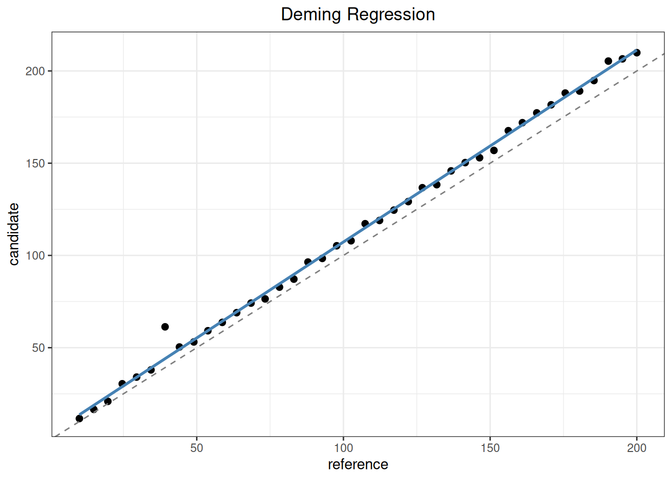

Code

plot(mc, type = "bland_altman")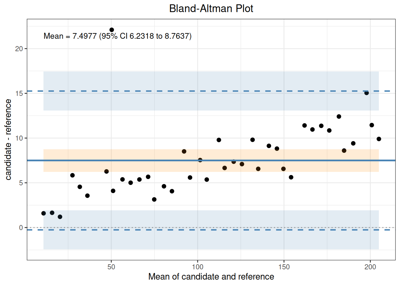

For subgroup analyses, split by lot or sample type using prespecified boundaries and repeat the same workflow on every subgroup. Do not let a pooled mean conceal subgroup-specific bias.

Code

rm_data <- as.data.frame(read_csv(
  "./data/009-方法学比较与参考物偏倚/std-wst408-reference-material.csv",
  show_col_types = FALSE
))
rm_fit <- reference_bias(
  rm_data,
  result = "result",
  reference = "assigned",
  reference_uncertainty = "expanded_uncertainty",
  level = "sample",
  k = 2
)
print(rm_fit)


Reference Material Bias
  Standard: YY/T 1789.2-2021, Section 5.3
  Data:     rm_data
  Result:   result
  Levels:   2
  Records:  20 valid, 0 excluded
  Coverage factor: k = 2

  Measurement and uncertainty
  Level: GBW09193
    n         : 10
    Mean      : 1.528
    SD        : 0.016193277
    Reference : 1.49
    U_ref     : 0.04
    u_X       : 0.0051207638
    U_X       : 0.010241528

  Level: GBW09195
    n         : 10
    Mean      : 1.05
    SD        : 0.014142136
    Reference : 1.02
    U_ref     : 0.04
    u_X       : 0.004472136
    U_X       : 0.0089442719

  Bias interval
  Level: GBW09193
    Bias                : 0.038
    Bias (%)            : 2.5503356
    Interval half-width : 0.0412903
    Lower               : -0.0032903002
    Upper               : 0.0792903

  Level: GBW09195
    Bias                : 0.03
    Bias (%)            : 2.9411765
    Interval half-width : 0.040987803
    Lower               : -0.010987803
    Upper               : 0.070987803

  Interval: Bias +/- sqrt(U_X^2 + U_ref^2)

9.4 Interpretation Checklist

Confirm candidate/reference direction and measurement units.
Use correlation only descriptively; interpret regression and Bland–Altman together.
Choose OLS, WLS, Deming, weighted Deming, or Passing–Bablok from the error structure.
Investigate, document, and sensitivity-test outliers.
Report bias at clinically relevant levels and compare it with prespecified limits.
Distinguish patient-sample agreement from reference-material bias and commutability.

9.5 Complete Standard Cases

9.5.1 Replicate Summaries and lambda

mcr() does not accept raw replicate rows with the same ID. First summarize both methods, then pass the mean columns as X/Y and the SD and n columns as replicate precision information. The two methods may have different replicate counts, but each count must be constant across samples; otherwise a single scalar lambda is not appropriate and a precision profile should be used.

Code

replicate_raw <- data.frame(
  sample = rep(1:8, each = 3),
  reference = rep(seq(10, 80, 10), each = 3) + rep(c(-1, 0, 1), 8),
  candidate = rep(2 + 1.05 * seq(10, 80, 10), each = 3) +
    rep(c(-0.5, 0, 0.5), 8)
)
replicate_summary <- replicate_to_mean(
  replicate_raw, "sample", c("candidate", "reference")
)
replicate_mcr <- mcr(
  replicate_summary,
  id = "x", candidate = "candidate_mean", reference = "reference_mean",
  candidate_sd = "candidate_sd", reference_sd = "reference_sd",
  candidate_n = "candidate_n", reference_n = "reference_n"
)
replicate_fit <- regression(
  replicate_mcr, method = "deming", lambda = "replicates"
)


Regression
  Method: Deming
  CI method: jackknife
  Lambda: 0.2500 (from summarized SD data)
  Intercept = 2.0000  (SE = 0.0000)
  Slope     = 1.0500  (SE = 0.0000)
  Intercept 95% CI: [2.0000, 2.0000]
  Slope     95% CI: [1.0500, 1.0500]
    H0: slope = 1 -> t = 170220065980364.3125, p = < 2.2e-16
    slope significantly different from 1 (CI excludes 1)
  Sigma     = 0.0000
  n = 8

9.5.2 CLSI EP09c Appendix C: Mixed Variance and Regression Models

Appendix C compares two reagent lots from the same measurement procedure using 79 samples. For samples 1–40, it uses the absolute difference Y − X; for samples 41–79, it uses the percentage difference Y − X relative to the mean of the two lots.

Code

ep09_c <- read_csv(
  "./data/009-方法学比较与参考物偏倚/std-ep09-appendix-c.csv",
  show_col_types = FALSE
)
ep09_c_diff <- mcr(
  as.data.frame(ep09_c),
  id = "id", candidate = "mp_y", reference = "mp_x"
)
ep09_c_diff <- describe(ep09_c_diff)


Descriptive Statistics
  Variable               n     Mean       SD      Min       Q1   Median       Q3      Max  NA
  --------------------------------------------------------------------------- 
    mp_x (X)            79   8.7969  16.2611   0.0010   0.1835   1.7730  11.5160  91.2350  
    mp_y (Y)            79   9.0292  17.4625   0.0010   0.1995   1.8330  11.5980  99.8020  
    Diff (Y-X)          79   0.2323   1.9178  -2.4890  -0.0515   0.0060   0.0760  13.3600  

  unit
  Level                Count  Percent
   -------------------------------------- 
  ug/L                    79   100.0%

Call bland_altman() separately for the low- and high-concentration groups prespecified in Appendix C. These groups are the samples numbered 1–40 and 41–79 in the study design. Their reference results overlap slightly at the boundary and cannot be reconstructed without loss by a single numeric cutpoint, so the data are split directly according to the study design rather than with split_by_cutpoints(). The low-concentration group uses absolute differences; for the high-concentration group, EP09c sets percent_denominator = “mean” to calculate Y − X relative to the mean of the two lots. x_axis controls the plotting position, while the percentage denominator controls the bias definition; they are separate parameters.

Code

ep09_c_low_mcr <- mcr(
  as.data.frame(ep09_c[1:40, ]),
  id = "id", candidate = "mp_y", reference = "mp_x"
)
ep09_c_low_mcr <- bland_altman(
  ep09_c_low_mcr, type = "difference", x_axis = "mean"
)


Bland-Altman
  Type:        difference
  Y-axis:      mp_y - mp_x
  X-axis:      Mean of mp_y and mp_x
  Method:       parametric
  n = 40

  Mean diff:       0.0204
  95% CI for mean diff: [-0.0101, 0.0509]
  SD diff:         0.0954
  95% LoA: [-0.1666, 0.2074]

  95% CI for LoA:
    Lower LoA: [-0.2192, -0.1140]
    Upper LoA: [0.1548, 0.2599]

Code

ep09_c_high_mcr <- mcr(
  as.data.frame(ep09_c[41:79, ]),
  id = "id", candidate = "mp_y", reference = "mp_x"
)
ep09_c_high_mcr <- bland_altman(
  ep09_c_high_mcr,
  type = "percent", x_axis = "mean", percent_denominator = "mean"
)


Bland-Altman
  Type:        percent
  Y-axis:      (mp_y - mp_x) / mean(mp_y, mp_x) * 100
  X-axis:      Mean of mp_y and mp_x
  Percent base: mean
  Method:       parametric
  n = 39

  Mean diff:       0.4303
  95% CI for mean diff: [-1.8286, 2.6892]
  SD diff:         6.9685
  95% LoA: [-13.2277, 14.0883]

  95% CI for LoA:
    Lower LoA: [-17.1215, -9.3339]
    Upper LoA: [10.1945, 17.9821]

EP09c Appendix C: segmented bias comparison
Standard location	Statistic	Standard	ivdtools
low_absolute	estimate	0.020	0.0204
low_absolute	lower	-0.010	-0.0101
low_absolute	upper	0.051	0.0509
high_percent	estimate	0.430	0.4303
high_percent	lower	-1.830	-1.8286
high_percent	upper	2.690	2.6892

Code

plot(ep09_c_low_mcr, type = "bland_altman")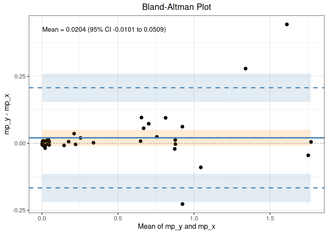

The orange band is the 95% CI for the mean difference; the blue bands are the 95% CIs for the lower and upper limits of agreement.

Fit the five models shown in standard Figures C(f)–C(j). weights = “constant_cv” uses 1/x^2 for WLS and the Linnet iterative constant-CV algorithm for weighted Deming; the latter refits the complete model after each jackknife deletion.

Code

ep09_c_mcr <- mcr(
  as.data.frame(ep09_c),
  id = "id", candidate = "mp_y", reference = "mp_x"
)
ep09_c_ols <- regression(ep09_c_mcr, method = "ols")


Regression
  Method: OLS
  CI method: analytic
  Intercept = -0.3804  (SE = 0.1995)
  Slope     = 1.0697  (SE = 0.0108)
  Intercept 95% CI: [-0.7777, 0.0169]
  Slope     95% CI: [1.0481, 1.0912]
    H0: slope = 1 -> t = 6.4219, p = 1.011e-08
    slope significantly different from 1 (CI excludes 1)
  R-squared = 0.9921
  Sigma     = 1.5576
  n = 79

Code

ep09_c_wls <- regression(
  ep09_c_mcr, method = "wls", weights = "constant_cv"
)


Regression
  Method: WLS
  Weights: constant_cv
  CI method: analytic
  Intercept = 0.0054  (SE = 0.0004)
  Slope     = 0.9238  (SE = 0.0521)
  Intercept 95% CI: [0.0046, 0.0062]
  Slope     95% CI: [0.8201, 1.0274]
    H0: slope = 1 -> t = -1.4642, p = 0.1472
    slope not significantly different from 1 (CI contains 1)
  R-squared = 0.8035
  Sigma     = 0.4456
  n = 79

Code

ep09_c_deming <- regression(ep09_c_mcr, method = "deming")


Regression
  Method: Deming
  CI method: jackknife
  Intercept = -0.4202  (SE = 0.1792)
  Slope     = 1.0742  (SE = 0.0367)
  Intercept 95% CI: [-0.7771, -0.0634]
  Slope     95% CI: [1.0012, 1.1472]
    H0: slope = 1 -> t = 2.0230, p = 0.04654
    slope significantly different from 1 (CI excludes 1)
  Sigma     = 1.5594
  n = 79

Code

ep09_c_wdeming <- regression(
  ep09_c_mcr, method = "wdeming", weights = "constant_cv"
)


Regression
  Method: Constant-CV Deming
  Weights: constant_cv
  CI method: jackknife
  Intercept = -0.0023  (SE = 0.0019)
  Slope     = 1.0372  (SE = 0.0264)
  Intercept 95% CI: [-0.0061, 0.0015]
  Slope     95% CI: [0.9846, 1.0899]
    H0: slope = 1 -> t = 1.4074, p = 0.1633
    slope not significantly different from 1 (CI contains 1)
  Sigma     = 0.0056
  n = 79

Code

ep09_c_pb <- regression(ep09_c_mcr, method = "pb")


Regression
  Method: Passing-Bablok
  CI method: rank
  Intercept = 0.0055  (SE = 0.0083)
  Slope     = 1.0028  (SE = 0.0132)
  Intercept 95% CI: [-0.0059, 0.0089]
  Slope     95% CI: [0.9830, 1.0162]
    H0: slope = 1 -> t = 0.2140, p = 0.8311
    slope not significantly different from 1 (CI contains 1)
  Sigma     = 1.9142
  n = 79

EP09c Appendix C: regression parameters
Standard location	Statistic	Standard	ivdtools
OLS	intercept	-0.3800	-0.3804
OLS	slope	1.0700	1.0697
WLS	intercept	0.0100	0.0054
WLS	slope	0.9200	0.9238
Deming	intercept	-0.4200	-0.4202
Deming	slope	1.0700	1.0742
Weighted Deming	intercept	0.0000	-0.0023
Weighted Deming	slope	1.0400	1.0372
Passing-Bablok	intercept	0.0055	0.0055
Passing-Bablok	slope	1.0028	1.0028

The constant-CV fit stores convergence, latent_concentration, and the final weights; internally it converts ppwdeming’s X/Y variance ratio to this package’s common Y/X lambda. Passing–Bablok follows Appendix I Algorithm I: it retains signed infinite slopes for vertical pairs, excludes slopes of −1, and applies the K shift.

Code

plot(ep09_c_pb, type = "regression")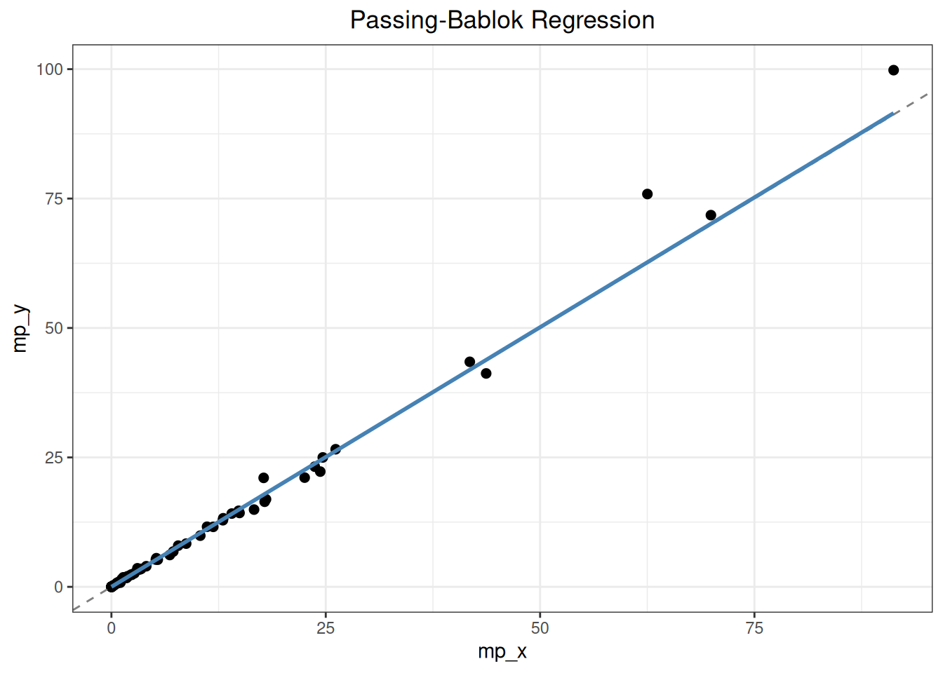

9.5.3 CLSI EP09c Appendix D: Six Data Patterns

The six Appendix D data sets each contain 40 paired results and illustrate how constant SD, constant CV, concentration distribution, and outliers affect difference plots and regression. The standard does not publish one uniform set of regression parameters for all six data sets, so the following OLS parameters are used only to verify the data structure.

Code

ep09_d <- read_csv(
  "./data/009-方法学比较与参考物偏倚/std-ep09-appendix-d.csv",
  show_col_types = FALSE
)
ep09_d_pattern <- c(
  D1 = "constant SD", D2 = "constant CV", D3 = "constant CV",
  D4 = "constant CV with outliers", D5 = "constant SD with outliers",
  D6 = "constant SD"
)

# Demonstrate the workflow on D4, which contains outliers, then use the
# same call for D1--D6 in the hidden summary below.
ep09_d4 <- as.data.frame(ep09_d[ep09_d$dataset == "D4", ])
ep09_d4_mcr <- mcr(
  ep09_d4, id = "sample",
  candidate = "candidate", reference = "comparative"
)
ep09_d4_mcr <- describe(ep09_d4_mcr)


Descriptive Statistics
  Variable               n     Mean       SD      Min       Q1   Median       Q3      Max  NA
  --------------------------------------------------------------------------- 
    comparative (X)     40 203.8413 226.8297   0.8810  31.6217 104.2190 282.3255 785.5660  
    candidate (Y)       40 224.5340 235.1985   1.0780  37.6600 140.9205 347.1503 801.2270  
    Diff (Y-X)          40  20.6928 107.4543 -205.3500  -2.0363   4.9985  18.7690 585.1470  

  dataset
  Level                Count  Percent
   -------------------------------------- 
  D4                      40   100.0%

Code

ep09_d4_mcr <- regression(ep09_d4_mcr, method = "ols")


Regression
  Method: OLS
  CI method: analytic
  Intercept = 35.9058  (SE = 22.9826)
  Slope     = 0.9254  (SE = 0.0759)
  Intercept 95% CI: [-10.6200, 82.4316]
  Slope     95% CI: [0.7717, 1.0790]
    H0: slope = 1 -> t = -0.9834, p = 0.3316
    slope not significantly different from 1 (CI contains 1)
  R-squared = 0.7965
  Sigma     = 107.4996
  n = 40

Code

plot(ep09_d4_mcr, type = "regression")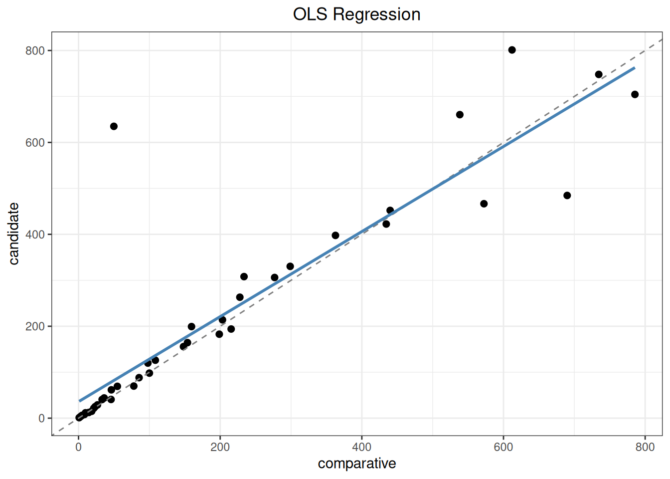

EP09c Appendix D: data structure and OLS diagnostics
	Dataset	Data pattern	Sample count	Intercept	Slope	Largest-residual sample
D1	D1	constant SD	40	9.1854	0.9959	29
D2	D2	constant CV	40	12.4287	0.9697	36
D3	D3	constant CV	40	7.3639	0.8942	39
D4	D4	constant CV with outliers	40	35.9058	0.9254	14
D5	D5	constant SD with outliers	40	0.5373	0.9594	3
D6	D6	constant SD	40	0.2171	1.0024	18

All six sets contain 40 complete pairs. Model choice should still be based on the error structure shown in the difference plot, not only on the correlation coefficient.

9.5.4 CLSI EP09c Appendix E: Generalized ESD Outlier Test

Appendix E uses the 100 relative biases from Appendix F to demonstrate generalized ESD with alpha = 0.01 and a maximum of five outliers. Relative bias is defined as 100 * (Y - X) / X.

Code

ep09_f <- read_csv(
  "./data/009-方法学比较与参考物偏倚/std-ep09-appendix-f.csv",
  show_col_types = FALSE
)
ep09_f_mcr <- mcr(
  as.data.frame(ep09_f),
  id = "id", candidate = "y", reference = "x"
)
ep09_e_result <- outlier(
  ep09_f_mcr, method = "esd", type = "percent", alpha = 0.01, r = 5
)


Outlier
  Method: esd
  Data:   Percent diff ((y - x) / x * 100)
  Alpha:  0.01

  1 outlier(s) found:
  Row                Value   Statistic  Critical
   -------------------------------------------------- 
  3               -55.7047      6.0896  3.7540

9.5.5 CLSI EP09c Appendix F: Median-Bias Intervals

Appendix F provides 100 paired results. The ordinary median demonstrates both the default conservative order-statistic interval and the continuous-rank interpolation interval; method = “hodges_lehmann” returns the Walsh-average pseudomedian and a Wilcoxon/Tukey interval without continuity correction. Nonparametric limits of agreement remain empirical quantiles with percentile-bootstrap intervals.

Code

ep09_f_ba <- bland_altman(
  ep09_f_mcr,
  type = "percent", x_axis = "reference",
  percent_denominator = "reference",
  method = "nonparametric", bootstrap_replicates = 1000, seed = 2026
)


Bland-Altman
  Type:        percent
  Y-axis:      (y - x) / x * 100
  X-axis:      x
  Percent base: reference
  Method:       nonparametric
  n = 100

  Median diff:     -0.3345
  95% requested CI for median diff (actual 96.5%): [-2.0202, 1.5873]
  SD diff:         9.1499
  95% LoA: [-12.6938, 16.2952]

  95% CI for LoA:
    Lower LoA: [-35.4958, -9.2515]
    Upper LoA: [11.6452, 22.4088]

Code

ep09_f_interpolated <- bland_altman(
  ep09_f_mcr,
  type = "percent", x_axis = "reference",
  percent_denominator = "reference",
  method = "nonparametric", median_ci_method = "interpolated",
  bootstrap_replicates = 1000, seed = 2026
)


Bland-Altman
  Type:        percent
  Y-axis:      (y - x) / x * 100
  X-axis:      x
  Percent base: reference
  Method:       nonparametric
  n = 100

  Median diff:     -0.3345
  95% requested CI for median diff (actual 95.0%): [-1.9970, 1.1783]
  SD diff:         9.1499
  95% LoA: [-12.6938, 16.2952]

  95% CI for LoA:
    Lower LoA: [-35.4958, -9.2515]
    Upper LoA: [11.6452, 22.4088]

Code

ep09_f_hl <- bland_altman(
  ep09_f_mcr,
  type = "percent", x_axis = "reference",
  percent_denominator = "reference",
  method = "hodges_lehmann",
  bootstrap_replicates = 1000, seed = 2026
)


Bland-Altman
  Type:        percent
  Y-axis:      (y - x) / x * 100
  X-axis:      x
  Percent base: reference
  Method:       hodges_lehmann
  n = 100

  HL pseudomedian: 0.0460
  95% CI for hl pseudomedian: [-1.4034, 1.6075]
  SD diff:         9.1499
  95% LoA: [-12.6938, 16.2952]

  95% CI for LoA:
    Lower LoA: [-35.4958, -9.2515]
    Upper LoA: [11.6452, 22.4088]

EP09c Appendix F: median-bias comparison
Standard location	Statistic	Standard	ivdtools
EP09c Appendix F	median	-0.335	-0.3345
EP09c Appendix F	position_40	-2.020	-2.0202
EP09c Appendix F	position_41	-1.990	-1.9871
EP09c Appendix F	position_60	1.000	1.0031
EP09c Appendix F	position_61	1.590	1.5873
EP09c Appendix F	interpolated_lower	-1.997	-1.9970
EP09c Appendix F	interpolated_upper	1.152	1.1783
EP09c Appendix F	HL_pseudomedian	-0.050	0.0460
EP09c Appendix F	HL_lower	-1.410	-1.4034
EP09c Appendix F	HL_upper	1.610	1.6075

The default median_diff_ci uses positions 40 and 61 to form a conservative order-statistic interval, with actual coverage of approximately 96.4%. The interpolated ranks are 40.7002 and 60.2998, giving −1.9970% to 1.1783% by linear interpolation of adjacent order statistics; the upper limit calculated from the public data differs from the 1.152% in the main text. Exact recalculation from Table F2 gives a Hodges–Lehmann pseudomedian of +0.05%, whereas the standard text reports −0.05%; the interval remains approximately −1.41% to 1.61%.

9.5.6 CLSI EP09c Appendix H: Iteratively Weighted Least Squares

Appendix H compares 120 platelet results from two analyzers. weights = “residual” first fits OLS, then estimates a linear SD function from absolute residuals and uses the inverse squared fitted SD as weights; weight_iterations = 4 updates the weights for four rounds as recommended by the standard.

Code

ep09_h <- read_csv(
  "./data/009-方法学比较与参考物偏倚/std-ep09-appendix-h.csv",
  show_col_types = FALSE
)
ep09_h_mcr <- mcr(
  as.data.frame(ep09_h),
  id = "sample", candidate = "candidate", reference = "comparative"
)
ep09_h_wls <- regression(
  ep09_h_mcr,
  method = "wls", weights = "residual", weight_iterations = 4
)


Regression
  Method: WLS
  Weights: residual
  Weight updates: 4
  CI method: analytic
  Intercept = 3.0202  (SE = 1.0724)
  Slope     = 1.0209  (SE = 0.0070)
  Intercept 95% CI: [0.8966, 5.1439]
  Slope     95% CI: [1.0071, 1.0347]
    H0: slope = 1 -> t = 2.9977, p = 0.003318
    slope significantly different from 1 (CI excludes 1)
  R-squared = 0.9945
  Sigma     = 1.2216
  n = 120


Regression
  Method: WLS
  Weights: residual
  Weight updates: 4
  CI method: analytic
  Intercept = 3.0202  (SE = 1.0724)
  Slope     = 1.0209  (SE = 0.0070)
  Intercept 95% CI: [0.8966, 5.1439]
  Slope     95% CI: [1.0071, 1.0347]
    H0: slope = 1 -> t = 2.9977, p = 0.003318
    slope significantly different from 1 (CI excludes 1)
  R-squared = 0.9945
  Sigma     = 1.2216
  n = 120

EP09c Appendix H: WLS comparison
Standard location	Statistic	Standard	ivdtools
EP09c Appendix H	intercept	3.013	3.0202
EP09c Appendix H	intercept_se	1.073	1.0724
EP09c Appendix H	intercept_lower	0.889	0.8966
EP09c Appendix H	intercept_upper	5.138	5.1439
EP09c Appendix H	slope	1.021	1.0209
EP09c Appendix H	slope_se	0.007	0.0070
EP09c Appendix H	slope_lower	1.007	1.0071
EP09c Appendix H	slope_upper	1.035	1.0347
EP09c Appendix H	regression_se	1.222	1.2216

The recalculated intercept is 3.020 versus 3.013 in the standard. Small interval differences may arise from unreported input precision or the standard’s recalculation process; they should not be interpreted as a different WLS formula.

9.5.7 CLSI EP09c Appendix I: Passing–Bablok Parameters and Bias Intervals

ci_method = “auto” selects the rank interval from Appendix I for Passing–Bablok regression parameters. Bias at a specified medical decision level is a joint function of the regression parameters.

Code

ep09_i_bias <- bias(
  ep09_c_pb, mdl = 1,
  interval = "confidence",
  bootstrap_replicates = 5000, seed = 202609
)


Bias
  Method: Passing-Bablok
  Interval: confidence (95%)
  MDL points: 1
  Bias range: [0.0083, 0.0083]

 mdl        bias    ci_lower   ci_upper 
--------------------------------------- 
   1 0.008343138 -0.01802986 0.02214245

The bias interval is obtained by resampling complete (X, Y) pairs; the point estimate remains the original Passing–Bablok fit. The returned object’s ci_method attribute is bootstrap_percentile.

9.5.8 CLSI EP09c Appendix J: Precision-Profile Weighted Deming

Appendix J requires the variance function for each method to be incorporated into the errors-in-variables regression. variance_models can receive functions that return variances or precision objects that have already been processed by variance() and profile(). Values outside the range of means in the precision study generate a warning; predicted nonpositive or nonfinite variances generate an error.

Code

ep09_j_precision_data <- read_csv(
  "./data/013-精密度分析/precision-profile.csv",
  show_col_types = FALSE
)
ep09_j_precision <- precision(
  as.data.frame(ep09_j_precision_data), value ~ day, by = "sample"
)

ep09_j_precision <- variance(ep09_j_precision)

Variance components
 sample component       VC %Total      SD  CV[%] Method
-------------------------------------------------------
     L1       day   0.6376   63.0  0.7985 3.9446  anova
     L1     error   0.3750   37.0  0.6124 3.0250  anova
     L2       day   5.7139   75.1  2.3904 4.7584  anova
     L2     error   1.8937   24.9  1.3761 2.7393  anova
     L3       day   3.3913   15.7  1.8415 1.8088  anova
     L3     error  18.1466   84.3  4.2599 4.1840  anova
     L4       day  30.5549   54.6  5.5276 2.7529  anova
     L4     error  25.4525   45.4  5.0451 2.5126  anova
     L5       day   0.0000    0.0  0.0000 0.0000  anova
     L5     error 171.7986  100.0 13.1072 3.3003  anova

Code

ep09_j_precision <- profile(ep09_j_precision)

Precision profiles -- Sadler
  total: sigma^2 = 0.0000 + 0.0086 * u^J  (AIC = 56.45, R^2 = 0.9847)
  day: sigma^2 = 0.0000 + 0.0095 * u^J  (AIC = 43.46, R^2 = 0.8919)
  error: sigma^2 = 0.0010 * u^2  (AIC = 55.96, R^2 = 0.9806)

Code

# Generate teaching data to demonstrate the analysis.
ep09_j_data <- data.frame(
  sample = 1:8,
  reference = seq(25, 350, length.out = 8)
)
ep09_j_data$candidate <- 1 + 1.03 * ep09_j_data$reference +
  c(-1.0, 0.8, -1.2, 1.1, -0.7, 0.9, -0.6, 0.7)

ep09_j_mcr <- mcr(
  ep09_j_data, "sample", "candidate", "reference"
)
ep09_j_profile_fit <- regression(
  ep09_j_mcr, method = "wdeming", weights = "precision_profile",
  variance_models = list(
    reference = ep09_j_precision,
    candidate = ep09_j_precision
  )
)


Regression
  Method: Precision-profile Deming
  Weights: precision_profile
  CI method: jackknife
  Intercept = 0.0131  (SE = 1.3393)
  Slope     = 1.0360  (SE = 0.0074)
  Intercept 95% CI: [-3.2639, 3.2902]
  Slope     95% CI: [1.0178, 1.0542]
    H0: slope = 1 -> t = 4.8363, p = 0.002892
    slope significantly different from 1 (CI excludes 1)
  Sigma     = 1.0955
  n = 8

9.5.9 CLSI EP09c Appendix K2: Regression and Bias Bootstrap

The percentile method takes parameter-sample quantiles directly. The standard method constructs intervals from the bootstrap standard error, intercept–slope covariance, and t(n-2). Each replicate resamples complete sample pairs and refits the selected model.

Code

ep09_k_percentile <- regression(
  ep09_c_mcr, method = "ols",
  ci_method = "bootstrap_percentile",
  bootstrap_replicates = 5000, seed = 202610, mdl = c(0.5, 2)
)


Regression
  Method: OLS
  CI method: bootstrap_percentile
  Bootstrap: 5000 effective / 5000 requested (0 failed)
  Intercept = -0.3804  (SE = 0.1738)
  Slope     = 1.0697  (SE = 0.0358)
  Intercept 95% CI: [-0.6645, 0.0425]
  Slope     95% CI: [0.9822, 1.1270]
    H0: slope = 1 -> t = 1.9441, p = 0.05554
    slope not significantly different from 1 (CI contains 1)
  R-squared = 0.9921
  Sigma     = 1.5576
  n = 79

Code

ep09_k_standard <- regression(
  ep09_c_mcr, method = "ols",
  ci_method = "bootstrap_standard",
  bootstrap_replicates = 5000, seed = 202610, mdl = c(0.5, 2)
)


Regression
  Method: OLS
  CI method: bootstrap_standard
  Bootstrap: 5000 effective / 5000 requested (0 failed)
  Intercept = -0.3804  (SE = 0.1738)
  Slope     = 1.0697  (SE = 0.0358)
  Intercept 95% CI: [-0.7265, -0.0343]
  Slope     95% CI: [0.9983, 1.1410]
    H0: slope = 1 -> t = 1.9441, p = 0.05554
    slope not significantly different from 1 (CI contains 1)
  R-squared = 0.9921
  Sigma     = 1.5576
  n = 79

Appendix K2: two bootstrap parameter intervals
method	parameter	estimate	lower	upper
percentile	intercept	-0.38040	-0.66451	0.04253
percentile	slope	1.06965	0.98218	1.12699
standard	intercept	-0.38040	-0.72652	-0.03428
standard	slope	1.06965	0.99831	1.14099

regression$bootstrap records the random seed, requested, valid, and failed replicate counts, and parameter_samples stores the joint parameter draws. When mdl is supplied during regression, bias draws are stored as well. bias() and predict() reuse draws from the same method. Prediction intervals are an ivdtools extension and should not be called EP09c regression-parameter or bias-confidence intervals.

9.5.10 YY/T 1789.2–2021 Appendix A: Reference-Material Bias

Appendix A uses national serum-cholesterol reference materials at three levels, with six replicate measurements at each level under repeatability conditions. reference_bias() combines expanded uncertainty of the measurement mean with reference-material uncertainty to form the bias interval.

Code

yyt_a <- read_csv(
  "./data/009-方法学比较与参考物偏倚/std-yyt1789-2-appendix-a.csv",
  show_col_types = FALSE
)
yyt_a_result <- reference_bias(
  as.data.frame(yyt_a),
  result = "result",
  reference = "assigned",
  reference_uncertainty = "reference_uncertainty",
  level = "level",
  k = 2
)
yyt_a_result


Reference Material Bias
  Standard: YY/T 1789.2-2021, Section 5.3
  Data:     as.data.frame(yyt_a)
  Result:   result
  Levels:   3
  Records:  18 valid, 0 excluded
  Coverage factor: k = 2

  Measurement and uncertainty
  Level: L1
    n         : 6
    Mean      : 192.35
    SD        : 0.60909769
    Reference : 197.6
    U_ref     : 2.5
    u_X       : 0.24866309
    U_X       : 0.49732618

  Level: L2
    n         : 6
    Mean      : 149.8
    SD        : 0.35777088
    Reference : 152.4
    U_ref     : 1.9
    u_X       : 0.14605935
    U_X       : 0.2921187

  Level: L3
    n         : 6
    Mean      : 119.5
    SD        : 0.42426407
    Reference : 122.1
    U_ref     : 1.6
    u_X       : 0.17320508
    U_X       : 0.34641016

  Bias interval
  Level: L1
    Bias                : -5.25
    Bias (%)            : -2.6568826
    Interval half-width : 2.5489867
    Lower               : -7.7989867
    Upper               : -2.7010133

  Level: L2
    Bias                : -2.6
    Bias (%)            : -1.7060367
    Interval half-width : 1.922325
    Lower               : -4.522325
    Upper               : -0.67767502

  Level: L3
    Bias                : -2.6
    Bias (%)            : -2.1294021
    Interval half-width : 1.6370706
    Lower               : -4.2370706
    Upper               : -0.96292945

  Interval: Bias +/- sqrt(U_X^2 + U_ref^2)

YY/T 1789.2 Appendix A: reference-material bias
Standard location	Statistic	Standard	ivdtools
Appendix A L1	mean	192.35	192.3500
Appendix A L1	sd	0.61	0.6091
Appendix A L1	standard_uncertainty	0.25	0.2487
Appendix A L1	expanded_uncertainty	0.50	0.4973
Appendix A L1	bias	-5.20	-5.2500
Appendix A L1	lower	-7.70	-7.7990
Appendix A L1	upper	-2.70	-2.7010
Appendix A L2	mean	149.80	149.8000
Appendix A L2	sd	0.36	0.3578
Appendix A L2	standard_uncertainty	0.15	0.1461
Appendix A L2	expanded_uncertainty	0.30	0.2921
Appendix A L2	bias	-2.60	-2.6000
Appendix A L2	lower	-4.50	-4.5223
Appendix A L2	upper	-0.70	-0.6777
Appendix A L3	mean	119.50	119.5000
Appendix A L3	sd	0.42	0.4243
Appendix A L3	standard_uncertainty	0.17	0.1732
Appendix A L3	expanded_uncertainty	0.34	0.3464
Appendix A L3	bias	-2.60	-2.6000
Appendix A L3	lower	-4.20	-4.2371
Appendix A L3	upper	-1.00	-0.9629

The means, SDs, uncertainties, and bias intervals at all three levels can be recalculated directly from the 18 raw results. At Level 1, the exact bias is −5.25 mg/dL while the standard displays −5.2 mg/dL; the exact lower bound of the combined interval is −7.80 mg/dL while the standard displays −7.7 mg/dL. These are differences caused by the standard’s stepwise display rounding.

9.5.11 YY/T 1789.2–2021 Appendix B: Patient-Sample Bias and Regression

Appendix B provides complete paired results for 120 patient samples. The comparative procedure is the X axis and the evaluated product is the Y axis. The standard analyzes the 75 samples with comparative results below 100 mg/dL using absolute differences and the 45 samples at or above 100 mg/dL using relative differences.

Code

yyt_b <- read_csv(
  "./data/009-方法学比较与参考物偏倚/std-yyt1789-2-appendix-b.csv",
  show_col_types = FALSE
)
head(yyt_b, 6)

# A tibble: 6 × 3
  sample comparative evaluated
   <dbl>       <dbl>     <dbl>
1      1          21        23
2      2         128       130
3      3          43        40
4      4         125       128
5      5         165       163
6      6         223       228

Code

yyt_b_data_list <- split_by_cutpoints(
  as.data.frame(yyt_b),
  variable = "comparative",
  cutpoints = 100,
  labels = c("low", "high")
)
yyt_b_data_list


Data split by cutpoints
  Variable: comparative
  Cutpoints: 100

  low        [-Inf, 100)           n = 75
  high       [100, Inf)            n = 45

Code

yyt_b_mcr <- lapply(
  yyt_b_data_list,
  \(d) mcr(
    d,
    id = "sample", candidate = "evaluated", reference = "comparative"
  )
)
yyt_b_mcr$low <- describe(yyt_b_mcr$low)


Descriptive Statistics
  Variable               n     Mean       SD      Min       Q1   Median       Q3      Max  NA
  --------------------------------------------------------------------------- 
    comparative (X)     75  60.4533  24.8647  12.0000  37.5000  65.0000  81.5000  98.0000  
    evaluated (Y)       75  62.2800  26.1847  13.0000  39.5000  67.0000  85.5000 104.0000  
    Diff (Y-X)          75   1.8267   3.6331  -7.0000  -1.5000   3.0000   4.0000   9.0000

Code

yyt_b_mcr$high <- describe(yyt_b_mcr$high)


Descriptive Statistics
  Variable               n     Mean       SD      Min       Q1   Median       Q3      Max  NA
  --------------------------------------------------------------------------- 
    comparative (X)     45 173.3111  45.8782 104.0000 129.0000 182.0000 199.0000 265.0000  
    evaluated (Y)       45 178.8444  48.9554 107.0000 132.0000 188.0000 207.0000 272.0000  
    Diff (Y-X)          45   5.5333   5.1416  -6.0000   3.0000   5.0000   7.0000  22.0000

Code

plot(yyt_b_mcr$low, type = "scatter")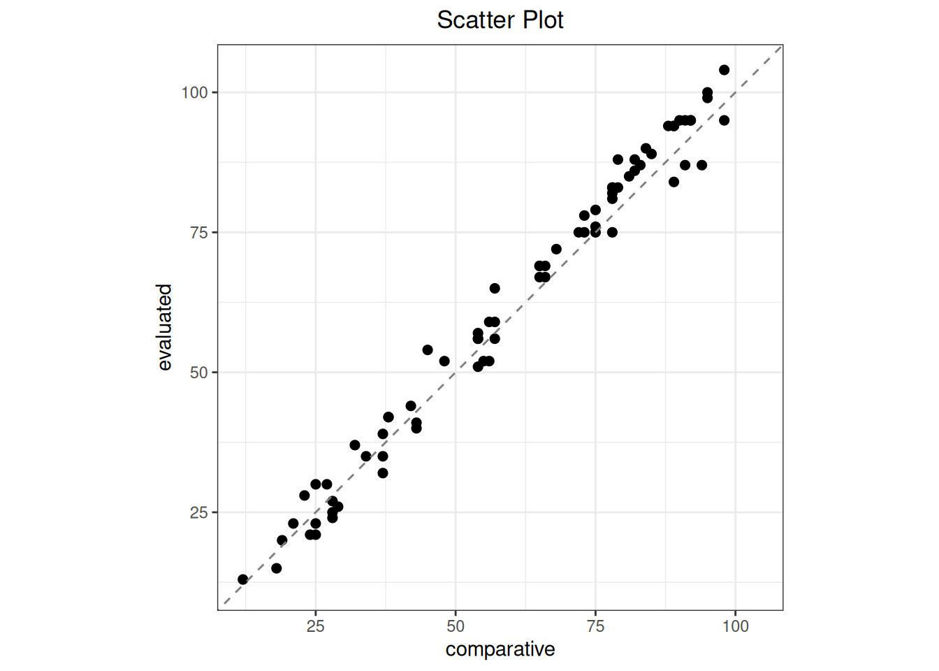

Code

plot(yyt_b_mcr$high, type = "scatter")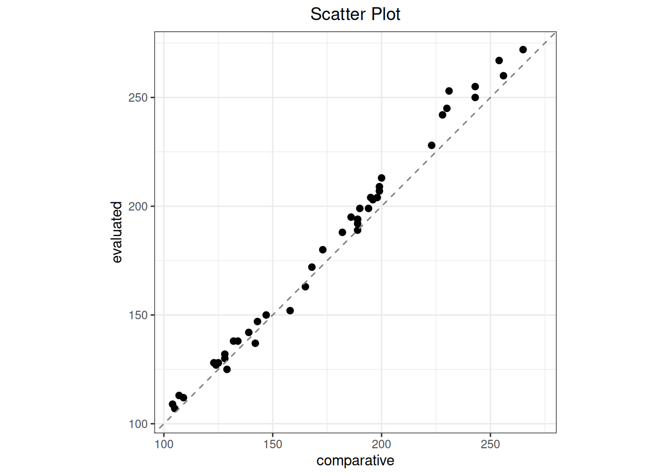

9.5.11.1 Generalized ESD Outlier Test

Difference analysis requires evaluated product minus comparative procedure, so the outlier objects pass the evaluated product as candidate.

Code

yyt_b_low_mcr <- yyt_b_mcr$low
yyt_b_high_mcr <- yyt_b_mcr$high
yyt_b_low_outlier <- outlier(
  yyt_b_low_mcr, method = "esd", type = "difference", alpha = 0.05, r = 3
)


Outlier
  Method: esd
  Data:   Difference (evaluated - comparative)
  Alpha:  0.05

  No outliers detected.

Code

yyt_b_high_outlier <- outlier(
  yyt_b_high_mcr, method = "esd", type = "percent", alpha = 0.05, r = 3
)


Outlier
  Method: esd
  Data:   Percent diff ((evaluated - comparative) / comparative * 100)
  Alpha:  0.05

  No outliers detected.

YY/T 1789.2 Appendix B: generalized ESD conclusions
interval	difference_scale	maximum_tests	detected_outliers
<100 mg/dL	absolute difference	3	0
>=100 mg/dL	relative difference	3	0

9.5.11.2 Segmented Bias

Call bland_altman() separately on the two prespecified mcr objects to obtain absolute differences in the low range and relative differences in the high range.

Code

yyt_b_low_ba <- bland_altman(
  yyt_b_low_mcr, type = "difference", x_axis = "mean"
)


Bland-Altman
  Type:        difference
  Y-axis:      evaluated - comparative
  X-axis:      Mean of evaluated and comparative
  Method:       parametric
  n = 75

  Mean diff:       1.8267
  95% CI for mean diff: [0.9908, 2.6626]
  SD diff:         3.6331
  95% LoA: [-5.2940, 8.9474]

  95% CI for LoA:
    Lower LoA: [-6.7289, -3.8591]
    Upper LoA: [7.5125, 10.3823]

Code

yyt_b_high_ba <- bland_altman(
  yyt_b_high_mcr, type = "percent", x_axis = "mean",
  percent_denominator = "reference"
)


Bland-Altman
  Type:        percent
  Y-axis:      (evaluated - comparative) / comparative * 100
  X-axis:      Mean of evaluated and comparative
  Percent base: reference
  Method:       parametric
  n = 45

  Mean diff:       3.0020
  95% CI for mean diff: [2.2441, 3.7600]
  SD diff:         2.5229
  95% LoA: [-1.9427, 7.9468]

  95% CI for LoA:
    Lower LoA: [-3.2477, -0.6377]
    Upper LoA: [6.6418, 9.2518]

YY/T 1789.2 Appendix B: segmented bias comparison
Standard location	Statistic	Standard	ivdtools
Appendix B low	mean_bias	1.8267	1.8267
Appendix B low	sd_bias	3.6331	3.6331
Appendix B low	lower	1.0000	0.9908
Appendix B low	upper	2.7000	2.6626
Appendix B high	mean_relative_bias	3.0000	3.0020
Appendix B high	sd_relative_bias	2.5230	2.5229
Appendix B high	lower	2.6000	2.2441
Appendix B high	upper	4.0000	3.7600

The confidence intervals differ somewhat because the statistical definitions are not identical.

9.5.11.3 Four Regression Models

The regression is evaluated-product-on-comparative-procedure, so the evaluated product is passed as candidate (Y) and the comparative procedure as reference (X). WLS uses weights = “residual” and iterates the standard’s absolute-residual SD function four times.

Code

yyt_b_reg_mcr <- mcr(
  as.data.frame(yyt_b),
  id = "sample", candidate = "evaluated", reference = "comparative"
)
yyt_b_ols <- regression(yyt_b_reg_mcr, method = "ols")


Regression
  Method: OLS
  CI method: analytic
  Intercept = -0.8416  (SE = 0.6630)
  Slope     = 1.0395  (SE = 0.0055)
  Intercept 95% CI: [-2.1545, 0.4713]
  Slope     95% CI: [1.0287, 1.0503]
    H0: slope = 1 -> t = 7.2214, p = 5.448e-11
    slope significantly different from 1 (CI excludes 1)
  R-squared = 0.9967
  Sigma     = 3.8533
  n = 120

Code

yyt_b_deming <- regression(yyt_b_reg_mcr, method = "deming")


Regression
  Method: Deming
  CI method: jackknife
  Intercept = -1.0230  (SE = 0.6625)
  Slope     = 1.0413  (SE = 0.0066)
  Intercept 95% CI: [-2.3348, 0.2889]
  Slope     95% CI: [1.0283, 1.0542]
    H0: slope = 1 -> t = 6.2964, p = 5.403e-09
    slope significantly different from 1 (CI excludes 1)
  Sigma     = 3.8550
  n = 120

Code

yyt_b_pb <- regression(yyt_b_reg_mcr, method = "pb")


Regression
  Method: Passing-Bablok
  CI method: rank
  Intercept = 0.0250  (SE = 0.7022)
  Slope     = 1.0375  (SE = 0.0075)
  Intercept 95% CI: [-0.8786, 1.0124]
  Slope     95% CI: [1.0248, 1.0485]
    H0: slope = 1 -> t = 4.9790, p = 2.204e-06
    slope significantly different from 1 (CI excludes 1)
  Sigma     = 3.9129
  n = 120

Code

yyt_b_wls <- regression(
  yyt_b_reg_mcr,
  method = "wls", weights = "residual", weight_iterations = 4
)


Regression
  Method: WLS
  Weights: residual
  Weight updates: 4
  CI method: analytic
  Intercept = -0.6980  (SE = 0.6193)
  Slope     = 1.0380  (SE = 0.0058)
  Intercept 95% CI: [-1.9243, 0.5283]
  Slope     95% CI: [1.0266, 1.0495]
    H0: slope = 1 -> t = 6.5761, p = 1.383e-09
    slope significantly different from 1 (CI excludes 1)
  R-squared = 0.9963
  Sigma     = 1.2988
  n = 120

YY/T 1789.2 Appendix B: regression parameters
Standard location	Statistic	Standard	ivdtools
Appendix B OLS	intercept	-0.842	-0.8416
Appendix B OLS	slope	1.039	1.0395
Appendix B WLS	intercept	-0.700	-0.6980
Appendix B WLS	slope	1.038	1.0380
Appendix B Deming	intercept	-1.023	-1.0230
Appendix B Deming	slope	1.041	1.0413
Appendix B Passing-Bablok	intercept	0.025	0.0250
Appendix B Passing-Bablok	slope	1.038	1.0375

The WLS intercept differs in the final displayed digits, possibly because of iteration stopping or display precision. The comparison retains both the standard and function values.

Code

plot(yyt_b_deming, type = "regression")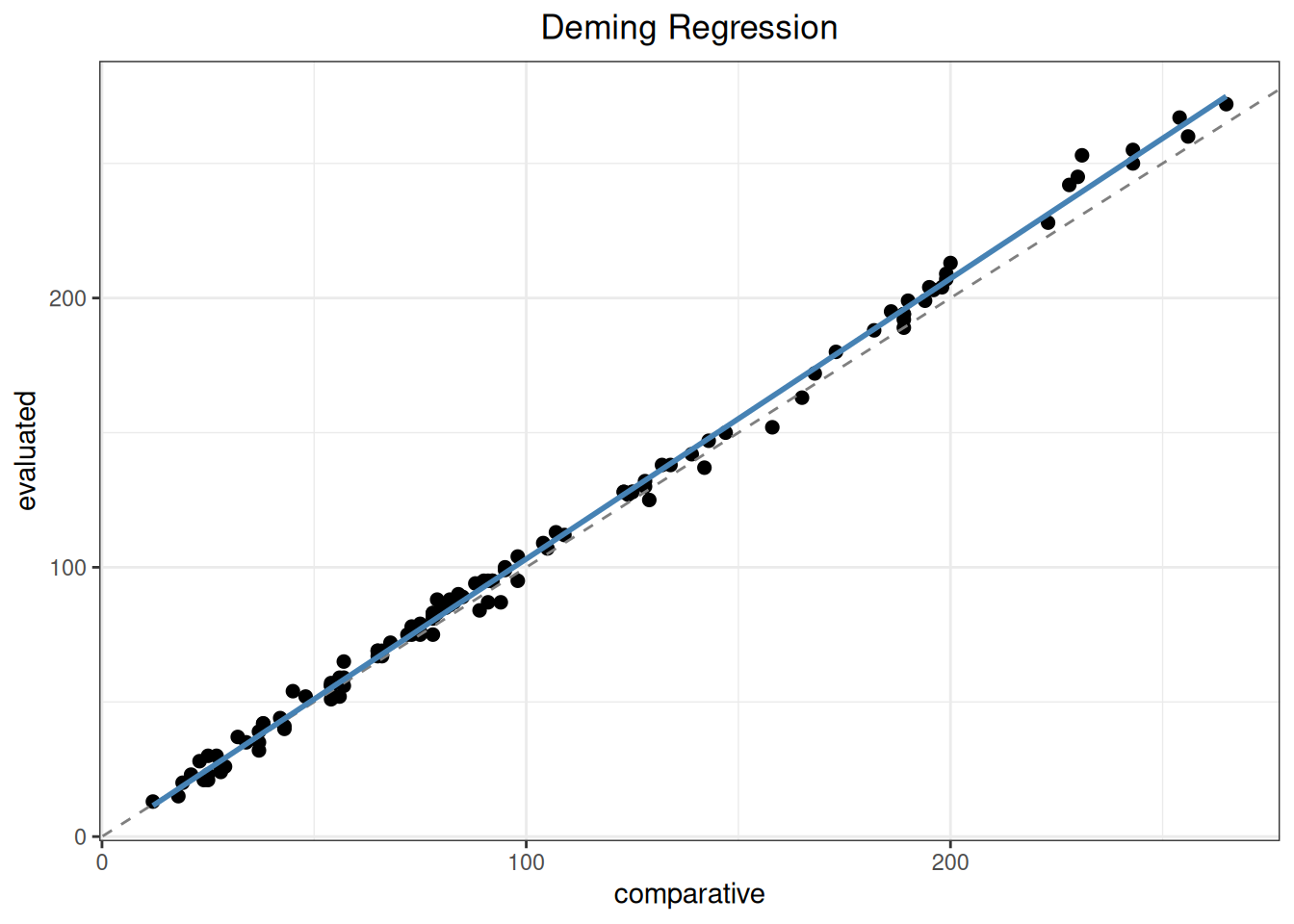

9.5.11.4 Bias at 125 mg/dL

The standard direction is evaluated product minus comparative procedure, namely intercept + (slope - 1) × 125, which is also bias()’s default direction.

Code

yyt_b_ols_bias <- bias(
  yyt_b_ols, mdl = 125, level = 0.95, interval = "confidence"
)


Bias
  Method: OLS
  Interval: confidence (95%)
  MDL points: 1
  Bias range: [4.0943, 4.0943]

 mdl     bias ci_lower ci_upper 
------------------------------- 
 125 4.094271 3.357293 4.831248

Code

yyt_b_wls_bias <- bias(
  yyt_b_wls, mdl = 125, level = 0.95, interval = "confidence"
)


Bias
  Method: WLS
  Interval: confidence (95%)
  MDL points: 1
  Bias range: [4.0575, 4.0575]

 mdl     bias ci_lower ci_upper 
------------------------------- 
 125 4.057517 3.271421 4.843613

Code

yyt_b_deming_bias <- bias(
  yyt_b_deming, mdl = 125, level = 0.95, interval = "confidence"
)


Bias
  Method: Deming
  Interval: confidence (95%)
  MDL points: 1
  Bias range: [4.1335, 4.1335]

 mdl     bias ci_lower ci_upper 
------------------------------- 
 125 4.133481 3.299802  4.96716

YY/T 1789.2 Appendix B: bias at 125 mg/dL
Standard location	Statistic	Standard	ivdtools
Appendix B OLS MDL	bias	4.1	4.0943
Appendix B OLS MDL	lower	3.4	3.3573
Appendix B OLS MDL	upper	4.8	4.8312
Appendix B WLS MDL	bias	4.1	4.0575
Appendix B WLS MDL	lower	3.5	3.2714
Appendix B WLS MDL	upper	4.7	4.8436
Appendix B Deming MDL	bias	4.1	4.1335
Appendix B Deming MDL	lower	3.4	3.2998
Appendix B Deming MDL	upper	4.9	4.9672

The WLS and Deming differences concern confidence-interval construction. The chapter retains the EP09c defaults and does not alter confidence level, random seed, or weight iterations to force agreement with a published value.

The WLS difference comes from whether the weighted-regression residual scale is applied a second time. YY/T 1789.2 Equation (8) uses

\[ SE\{\widehat B(x_c)\} = \sqrt{ \frac{1}{\sum_i w_i} + \frac{(x_c-\bar x_w)^2}{SSX_w} }. \]

It does not multiply by the weighted residual scale $S_{y\cdot x}$. Here the degrees of freedom are 118, $t_{0.975,118}=1.980272$, the bias estimate is 4.057517 mg/dL, and the Equation (8) SE is 0.305646 mg/dL. The half-width is 0.605262 mg/dL, giving 3.4523–4.6628 mg/dL, displayed as 3.5–4.7 mg/dL.

The ivdtools WLS analytic interval agrees with EP09c Appendix H H17–H18 and multiplies that SE by $S_{y\cdot x}$. Here $S_{y\cdot x}=1.298770$, giving adjusted SE 0.396964 mg/dL, half-width 0.786096 mg/dL, and interval 3.2714–4.8436 mg/dL. The half-width ratio is exactly 1.298770, so this is a formula choice about residual-scale correction, not random variation or decimal rounding. If weights are known absolute inverse variances from an independent precision study, the Equation (8) expression has a clear model basis; with weights iteratively estimated from the same residuals, residual-scale correction is more defensible. The standard also uses $S_{y\cdot x}$ for WLS regression-parameter SEs but not for Equation (8), so the two scale conventions differ.

For Deming, the bias SE uses intercept, slope, and covariance:

\[ SE\{\widehat B(x_c)\} = \sqrt{ \widehat\sigma_a^2+x_c^2\widehat\sigma_b^2 +2x_c\widehat\sigma_{ab} }. \]

YY/T 1789.2 uses its analytic covariance formula, whereas ci_method = “auto” in ivdtools follows EP09c Appendix K1: delete each sample, refit Deming, and calculate the covariance from 120 leave-one-out parameter sets. Here the bias estimate is 4.133481 mg/dL and the jackknife SE is 0.420992 mg/dL; the t multiplier gives a half-width of 0.833679 mg/dL and interval 3.2998–4.9672 mg/dL. YY/T 1789.2 publishes 3.4–4.9 mg/dL. Both intervals have explicit assumptions and should be reported as methodological differences, not calculation errors or simple rounding differences.