Code
library(ivdtools)
library(readr)Stability studies evaluate how measurement results change over time for reagents, calibrators, or QC materials under specified storage, transport, or use conditions. This chapter covers study planning, node bias, trends within and between conditions, time to an allowable limit, Arrhenius accelerated stability, and mean kinetic temperature (MKT).
Teaching data and illustrative limits in this chapter are deterministic examples, not universal acceptance criteria. Formal studies must use parameters specified by the protocol, risk assessment, and applicable standards. Decide in advance whether the response is concentration or signal, the time unit, bias scale, change direction, and allowable limit.
library(ivdtools)
library(readr)| Function | Main purpose | Key result |
|---|---|---|
stability_plan() |
Plan the minimum number of time points | Drift, variability, replicates, expected drift, power |
stability_bias() |
Calculate bias from the first node and between conditions | Node summaries and limit status |
stability_regression() |
Regress a single-condition trend or paired test/reference bias | Slope, one-sided limit, node results, diagnostics |
stability_time() |
Predict when a point estimate or one-sided limit reaches an allowable bias | Predicted time and extrapolation status |
arrhenius() |
Extrapolate target-temperature shelf life from elevated temperatures | Kinetic order, rate, activation energy, shelf life |
mkt() |
Calculate equally spaced or time-weighted mean kinetic temperature | Per-probe and combined MKT |
stability_regression() has two modes: mode="self" regresses one condition over time; mode="compare" calculates test-versus-reference bias at matched times and regresses the bias.
Suppose the protocol specifies an allowable relative drift of 5%, an expected drift of 2.5%, repeatability variability of 1.5%, and a target power of 90%. Compare the minimum number of time points required when 1, 2, or 3 replicates are measured at each time point:
plan <- stability_plan(
  allowable_drift = 5,
  variability = 1.5,
  replicates = c(1, 2, 3),
  expected_drift = 2.5,
  power = 0.9,
  mode = "simple",
  bias_type = "relative"
)
print(plan)
Stability Study Time-Point Plan
  Allowable drift: 5.0000; expected drift: 2.5000
  Success target:  90%; method: CLSI EP25 Appendix A Table A2

  Replicates     Residual  Allow/Resid  Min nodes
  ------------------------------------------------
           1       1.5000       3.3333        n/a
           2       1.0607       4.5455         28
           3       0.8660       5.7471         18

  n/a -- No feasible entry in EP25 table.
allowable_drift must be positive. In simple mode, variability is a relative CV/SD; in components mode, it can be a data frame of variance components. replicates can contain one or more replicate counts per time point. The returned stability_plan object provides time-point/sample-size recommendations for the requested power and replicate counts.
Read the raw data:
bias_data <- read_csv(
  "./data/004-稳定性研究/stability-bias-example.csv",
  show_col_types = FALSE
)
bias_result <- stability_bias(
  data = bias_data, condition = "Condition", time = "Day",
  value = "Result", reference_condition = "2-8C", limit = 5,
  bias_type = "relative", time_unit = "d"
)
print(bias_result)
Stability Bias Analysis
  Conditions:      2 (2-8C, 25C)
  Reference:       2-8C
  Time unit:       d
  Node comparisons:20
  Acceptance:      +/- 5.0000 (relative); 10/10 nodes passed

  Within-condition bias (vs first node)
  Cond         Time      Value    Bias(%) Status
  ----------------------------------------------
  2-8C       0.0000   100.0000     0.0000 Pass
  2-8C       7.0000    99.9333    -0.0667 Pass
  2-8C      14.0000    99.7333    -0.2667 Pass
  2-8C      21.0000    99.5000    -0.5000 Pass
  2-8C      28.0000    99.3333    -0.6667 Pass
  25C        0.0000   100.0000     0.0000 Pass
  25C        7.0000    99.2333    -0.7667 Pass
  25C       14.0000    98.3333    -1.6667 Pass
  25C       21.0000    97.2333    -2.7667 Pass
  25C       28.0000    95.8333    -4.1667 Pass

  Between-condition bias (reference: 2-8C)
      Time Condition    TestVal  Bias(%)
  --------------------------------------
    0.0000 25C        100.0000     0.0000
    7.0000 25C         99.2333    -0.7005
   14.0000 25C         98.3333    -1.4037
   21.0000 25C         97.2333    -2.2781
28.0000 25C 95.8333 -3.5235plot(bias_result)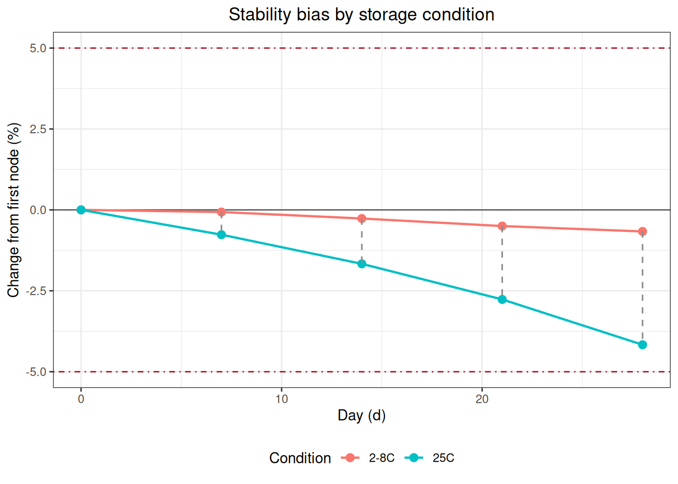
The function summarizes the mean by condition and time and returns a stability_bias object containing node means, relative/absolute bias, the reference condition, and limit status. When reference_condition = NULL, the software selects a reference according to data order; formal analyses should specify it explicitly. Missing or non-finite observations are removed, and the cleaning record must be retained. Within-condition bias uses each condition’s first node as its baseline; between-condition bias compares the test and reference conditions at matched time points.
Read the raw data:
regression_data <- read_csv(
  "./data/004-稳定性研究/stability-regression-example.csv",
  show_col_types = FALSE
)
regression_result <- stability_regression(
  data = regression_data, time = "Day", value = "Result",
  condition = "Condition", mode = "compare", test_condition = "25C",
  reference_condition = "2-8C", bias_type = "relative", direction = "decrease",
  conf.level = 0.95, limit = 5, time_unit = "d"
)
print(regression_result)
Stability Regression
  Mode:            compare
  Test condition:  25C
  Reference:       2-8C
  Fit:             WLS (1/SE^2); intercept = 0.0799, slope = -0.1025
  Direction:       decrease
  One-sided CI:    95.0%
  R-squared:       0.9956
  Cook distance:   row(s) 6 > 1; not removed

      Time      ObsBias   Estimate   CI_limit Status
  --------------------------------------------------
    0.0000       0.0000     0.0799    -0.0750
    7.0000      -0.6669    -0.6376    -0.7566
   14.0000      -1.3013    -1.3552    -1.4522
   21.0000      -2.0040    -2.0728    -2.1717
   28.0000      -2.6747    -2.7904    -2.9140
42.0000 -4.3842 -4.2256 -4.4296 plot(regression_result)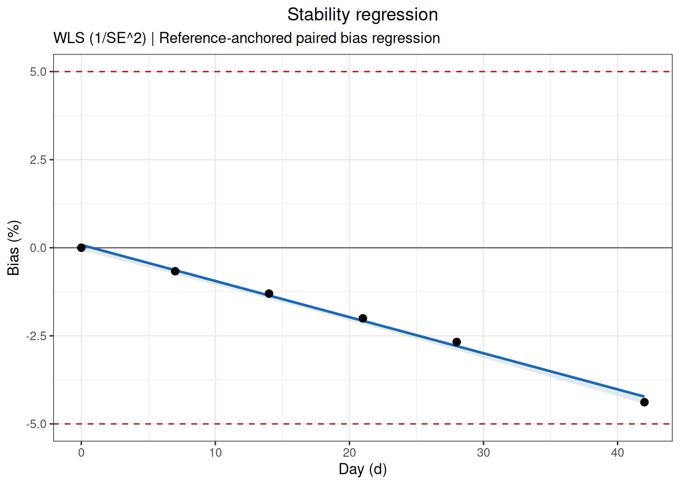
The one-sided confidence limit evaluates the prespecified least-favorable direction. A large Cook’s distance is a diagnostic flag, not an automatic exclusion; review records and perform inclusion/exclusion sensitivity analysis when justified.
For a single condition relative to its first node, use mode="self" and test_condition. The observed first-node bias is fixed at zero, but a fitted regression line need not pass exactly through that point.
At each matched time point, calculate the relative bias of 25C against 2-8C and regress the bias over time. The example prespecifies a decreasing response, so it uses direction = "decrease".
mode = "self" uses the first node of one condition as the reference; mode = "compare" compares a test condition with a reference condition. With direction = "auto", the direction is inferred from the slope; a formal protocol should preferably specify decrease or increase explicitly. With limit = NULL, the model is fitted without an acceptance status.
The returned stability_regression object includes the fitted model, slope/intercept, direction, bias scale, confidence limits, observed time range, condition mapping, and exclusions. Use print() for a summary and plot() for the trend, bias, and confidence limit.
This example identifies a node with a large Cook’s distance, but the function does not delete it automatically. Review the original records, experimental process, and protocol, and perform sensitivity analyses with and without the node only when justified.
stability_regression()mode = "self" analyzes the change of one condition over time. The following example uses the regression data but selects only the 25C condition; each node’s observed_bias is calculated relative to the mean of the first node:
self_regression_result <- stability_regression(
  data = regression_data,
  time = "Day",
  value = "Result",
  condition = "Condition",
  mode = "self",
  test_condition = "25C",
  bias_type = "relative",
  direction = "decrease",
  conf.level = 0.95,
  limit = 5,
  time_unit = "d"
)
print(self_regression_result)
Stability Regression
  Mode:            self
  Test condition:  25C
  Fit:             WLS (1/SE^2); intercept = 100.0849, slope = -0.1115
  Direction:       decrease
  One-sided CI:    95.0%
  R-squared:       0.9966
  Cook distance:   row(s) 1, 6 > 1; not removed

      Time      ObsBias   Estimate   CI_limit Status
  --------------------------------------------------
    0.0000       0.0000    -0.0000    -0.0000
    7.0000      -0.7000    -0.7797    -0.8278
   14.0000      -1.4000    -1.5594    -1.6555
   21.0000      -2.2000    -2.3391    -2.4833
   28.0000      -2.9667    -3.1188    -3.3110
42.0000 -4.7667 -4.6782 -4.9665 plot(self_regression_result)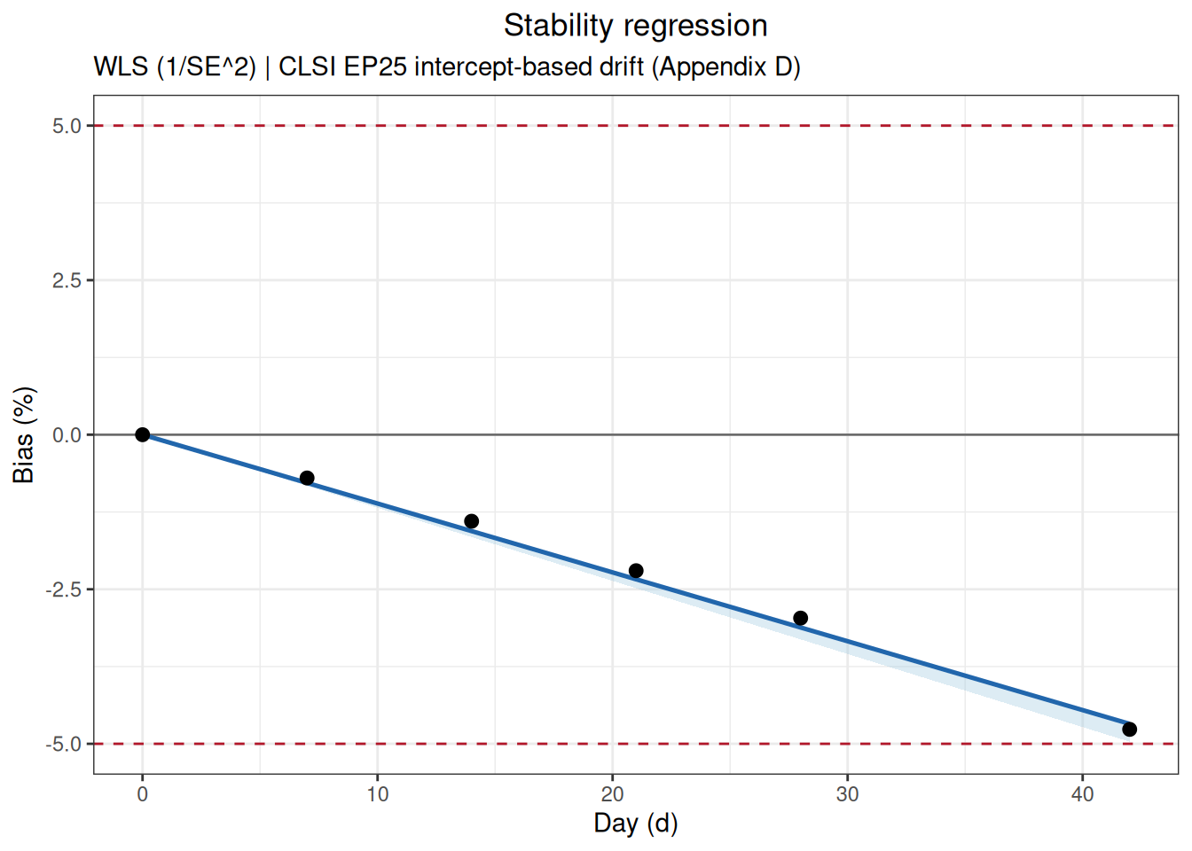
The observed bias at the first node is fixed at 0. The model estimate is fitted jointly from all time points, so the regression intercept is not required to pass exactly through that node.
stability_time() calculates separately the time when the point estimate and the one-sided confidence limit first reach a bias of −5%:
time_result <- stability_time(regression_result, limit = 5, max_time = 90)
print(time_result)
Stability Limit Time
  Limit: 5.0000 (relative); direction: decrease
  estimate       49.5548 d [EXTRAPOLATED]
one_sided_ci 47.2316 d [EXTRAPOLATED]plot(time_result)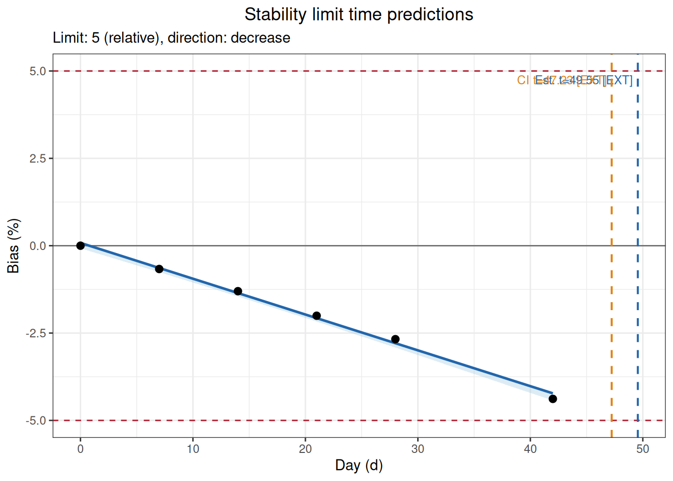
If the predicted time lies beyond the longest observed time, the result is marked EXTRAPOLATED. Extrapolation assumes that the trend continues and is not equivalent to observed stability evidence.
The input must be a stability_regression object. The function evaluates the first time at which the point estimate or one-sided confidence limit reaches the threshold, returns a stability_time object, and marks whether the result is beyond the observed range. max_time is only a search bound, not a scientifically justified shelf life; substantial extrapolation requires separate justification.
The longest observed time in this example is 42 days, while the predicted limit time is beyond the observed range, so the output is marked EXTRAPOLATED. The extrapolation assumes that the linear trend continues outside the observed interval and is not equivalent to measured stability evidence. Report the extrapolation distance and uncertainty clearly, and preferably confirm it with longer real-time observations.
Read and inspect the raw data:
arrhenius_data <- read_csv(
  "./data/004-稳定性研究/stability-arrhenius-example.csv",
  show_col_types = FALSE
)
arrhenius_result <- arrhenius(
  data = arrhenius_data, temperature = "Temperature", time = "Day",
  value = "Result", target_temp = 5, order = "auto", direction = "decrease",
  limit = 10, bias_type = "relative", temp_unit = "C", time_unit = "d",
  conf.level = 0.95
)
print(arrhenius_result)
Arrhenius Stability Analysis
  Kinetic order:   zero (auto-selected)
  Direction:       decrease
  Activation Ea:   97.159 kJ/mol
  Target rate:     0.002346 /d
Limit time: 4263.7878 d [1585.3589, 11467.3633]plot(arrhenius_result)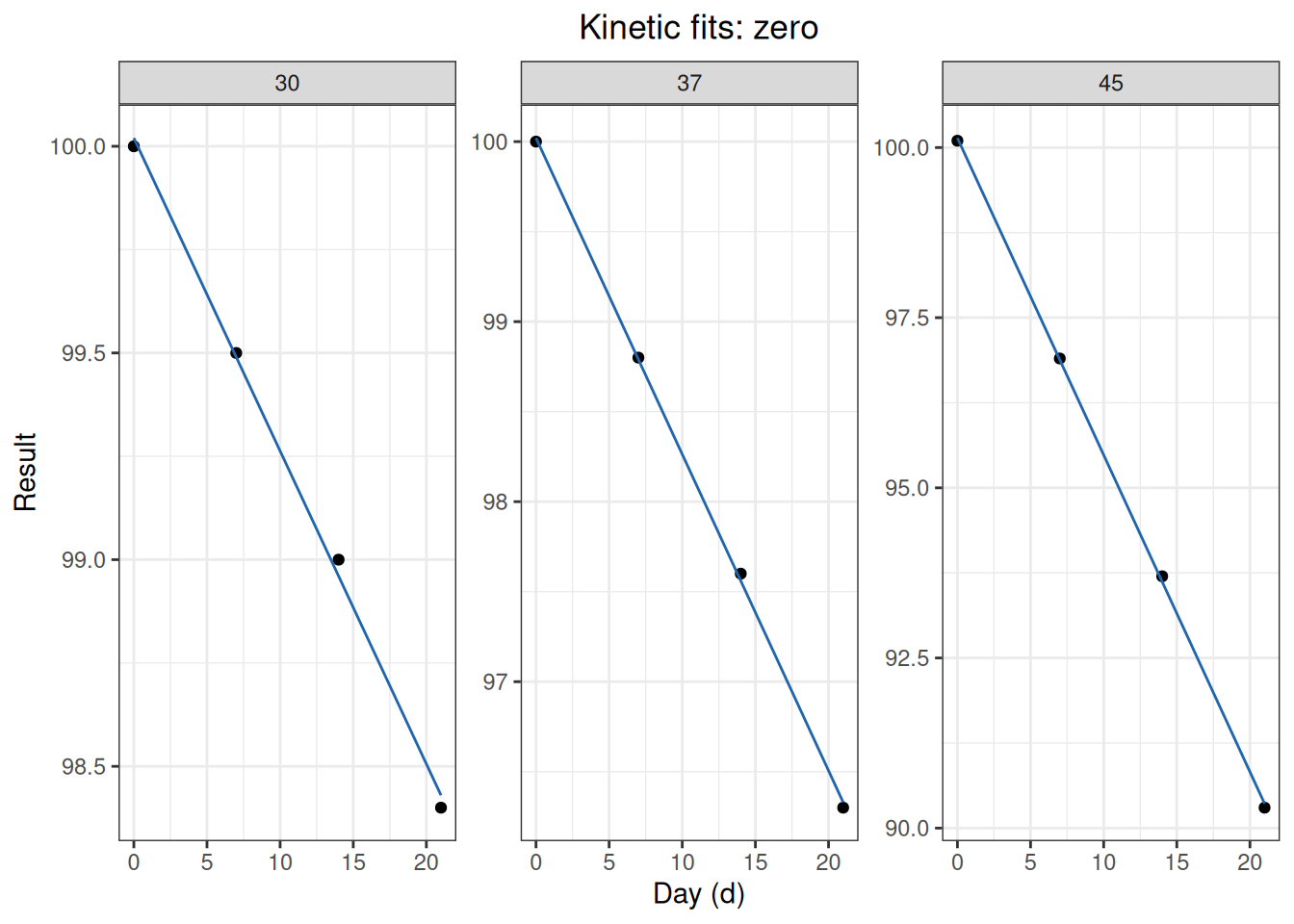
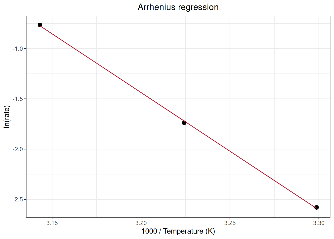
order="auto" selects from zero- and first-order candidates under the implementation rules. Formal work should justify kinetic order, degradation direction, rate significance, extent of degradation, residuals at each temperature, and the potentially large extrapolation to the target temperature.
mkt_data <- read_csv(
  "./data/004-稳定性研究/stability-mkt-example.csv",
  show_col_types = FALSE
)
mkt_data$Timestamp <- as.POSIXct(
  mkt_data$Timestamp, format = "%Y-%m-%d %H:%M:%S", tz = "UTC"
)
mkt_result <- mkt(
  data = mkt_data, temp_cols = c("Probe_A", "Probe_B"),
  time = "Timestamp", temp_unit = "C", ea = 83.144
)
print(mkt_result)
Mean Kinetic Temperature
  Ea: 83.144 kJ/mol
  Method: Time-weighted trapezoidal MKT

  Probe_A              299.538 K     26.388 C
  Probe_B              299.194 K     26.044 C
  Combined             299.367 K     26.217 C
MKT is not an arithmetic temperature mean; high temperatures receive greater weight through the Arrhenius relationship. Confirm probe calibration, time ordering, missing intervals, temperature units, exposure duration, and activation energy. MKT summarizes exposure and cannot replace a product-specific stability study.
mkt() returns the mean kinetic temperature for each probe and for the combined series. When time is supplied, observations are weighted by their time intervals; otherwise equal spacing is assumed. ea is the assumed activation energy in kJ/mol and must be reported.
When different concentration levels, sample types, or lots must be evaluated separately, retain the sample identifier, split the data first, and analyze each sample with the same prespecified parameters. Read and inspect the multiple-sample data:
multiple_samples_data <- read_csv(
  "./data/004-稳定性研究/stability-multiple-samples-example.csv",
  show_col_types = FALSE
)
head(multiple_samples_data, 6)
# A tibble: 6 × 4
Sample Day Replicate Result
<chr> <dbl> <dbl> <dbl>
1 Sample_A 0 1 100.
2 Sample_A 0 2 99.8
3 Sample_A 0 3 100
4 Sample_A 7 1 99.7
5 Sample_A 7 2 99.5
6 Sample_A 7 3 99.8Use split_by_factors() to build a named list by a classification column. The function keeps the split column, uses the observed sample values as list names, and reports the number of rows in each group and the rows excluded because the grouping value was missing:
sample_data_list <- split_by_factors(
  multiple_samples_data,
  variable = "Sample"
)
sample_data_list
Data split by factors
  Variable: Sample
  Groups: 2
  Missing/excluded: 0

  Sample_A  n = 18
Sample_B n = 18sample_a_data <- sample_data_list[["Sample_A"]]Then run the analysis for each sample.
Appendix B provides accelerated-stability data for a control material at 40, 45, 50, and 55 °C. The target storage temperature is 25 °C and the allowable decrease is 20%. The standard first log-transforms the results at each temperature and fits first-order kinetics, then uses the Arrhenius model to extrapolate the reaction rate and shelf life at 25 °C.
Read and inspect the raw data:
ep25_b_data <- read_csv(
  "./data/004-稳定性研究/std-ep25-appendix-b.csv",
  show_col_types = FALSE
)
head(ep25_b_data, 6)
# A tibble: 6 × 3
Temperature Day Result
<dbl> <dbl> <dbl>
1 40 0 1.02
2 40 10 0.956
3 40 21 0.945
4 40 31 0.933
5 40 42 0.908
6 40 52 0.86 Analyze with the first-order model, decreasing direction, 20% allowable change, and 25 °C target temperature specified by Appendix B:
ep25_b_result <- arrhenius(
  data = ep25_b_data,
  temperature = "Temperature",
  time = "Day",
  value = "Result",
  target_temp = 25,
  order = "first",
  direction = "decrease",
  limit = 20,
  bias_type = "relative",
  temp_unit = "C",
  time_unit = "d",
  conf.level = 0.95
)
print(ep25_b_result)
Arrhenius Stability Analysis
  Kinetic order:   first
  Direction:       decrease
  Activation Ea:   80.160 kJ/mol
  Target rate:     0.000582 /d
  Limit time:      383.1423 d [330.8315, 443.7244]
WARNING: Observed degradation exceeds 20% at one or more temperatures.plot(ep25_b_result)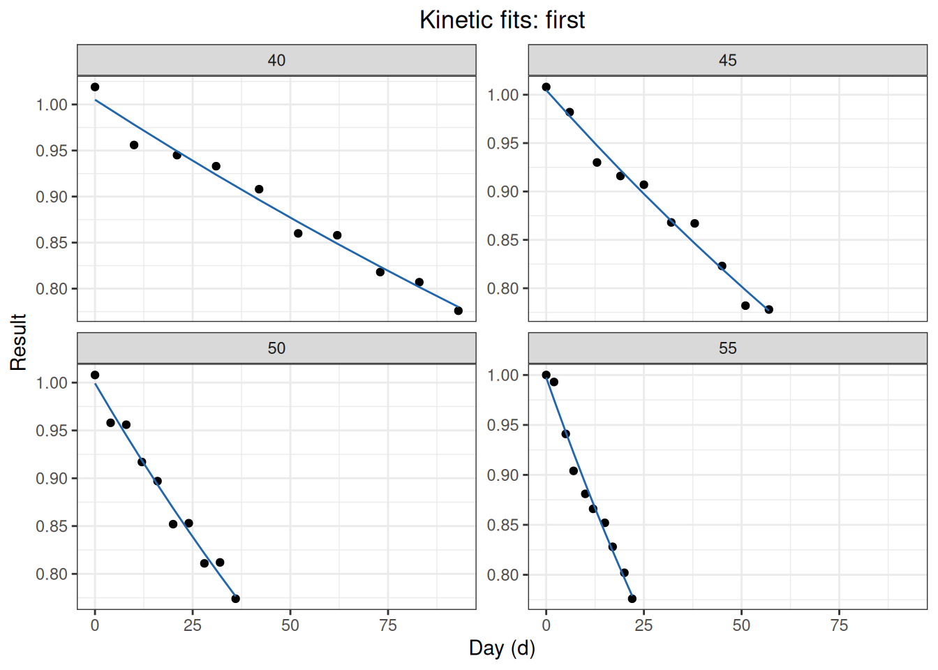
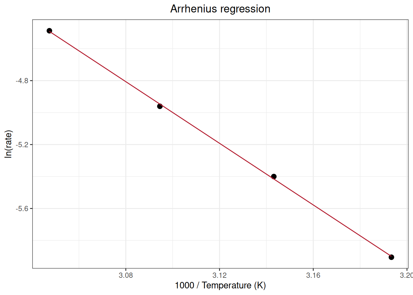
Extract the degradation rates at each temperature, the Arrhenius regression coefficients, the target rate at 25 °C, and the shelf life from the arrhenius() result, then compare them with the values reported in Appendix B:
| appendix | statistic | standard | ivdtools |
|---|---|---|---|
| EP25-A2 Appendix B / 40C | rate | 2.7257e-03 | 0.0027257 |
| EP25-A2 Appendix B / 45C | rate | 4.5154e-03 | 0.0045154 |
| EP25-A2 Appendix B / 50C | rate | 7.0087e-03 | 0.0070087 |
| EP25-A2 Appendix B / 55C | rate | 1.1243e-02 | 0.0112430 |
| EP25-A2 Appendix B / Arrhenius | slope | -9.6320e+03 | -9640.9966367 |
| EP25-A2 Appendix B / Arrhenius | intercept | 2.4874e+01 | 24.8877147 |
| EP25-A2 Appendix B / 25C | target_rate | 5.8250e-04 | 0.0005824 |
| EP25-A2 Appendix B / 25C | shelf_life | 3.8300e+02 | 383.1423039 |
Appendix C1 contains single-lot reagent data covering 0–418 days, with a claimed period of 364 days and an allowable drift of 10%. Each of the three series is represented by the mean at each time point; here they are analyzed with stability_regression() in self mode, using relative bias and a decreasing direction.
ep25_c1 <- read_csv(
  "./data/004-稳定性研究/std-ep25-appendix-c1.csv",
  show_col_types = FALSE
)
head(ep25_c1, 6)
# A tibble: 6 × 3
series day result
<chr> <dbl> <dbl>
1 low_panel 0 7.07
2 low_panel 33 6.95
3 low_panel 61 6.99
4 low_panel 95 6.88
5 low_panel 121 6.98
6 low_panel 155 6.83ep25_c1_list <- split_by_factors(
ep25_c1,
variable = "series"
)
ep25_c1_list
Data split by factors
  Variable: series
  Groups: 3
  Missing/excluded: 0

  low_panel     n = 13
  low_control   n = 13
  high_control  n = 13
Analyze the series with stability_regression():
ep25_low_panel <- stability_regression(
  ep25_c1_list$low_panel,
  time = "day", value = "result", mode = "self",
  bias_type = "relative", direction = "decrease",
  conf.level = 0.95, limit = 10, time_unit = "d"
)

ep25_low_control <- stability_regression(
  ep25_c1_list$low_control,
  time = "day", value = "result", mode = "self",
  bias_type = "relative", direction = "decrease",
  conf.level = 0.95, limit = 10, time_unit = "d"
)

ep25_high_control <- stability_regression(
  ep25_c1_list$high_control,
  time = "day", value = "result", mode = "self",
  bias_type = "relative", direction = "decrease",
  conf.level = 0.95, limit = 10, time_unit = "d"
)
Compare the calculated results with the values reported in the standard:
| appendix | statistic | standard | ivdtools |
|---|---|---|---|
| EP25-A2 Appendix C1 / low_panel | slope | -0.001567 | -0.001567 |
| EP25-A2 Appendix C1 / low_panel | intercept | 7.065000 | 7.065100 |
| EP25-A2 Appendix C1 / low_panel | change_364 | -8.070000 | -8.074378 |
| EP25-A2 Appendix C1 / low_panel | change_364_upper_CL | -9.260000 | -9.262841 |
| EP25-A2 Appendix C1 / low_panel | change_418 | -9.270000 | -9.272226 |
| EP25-A2 Appendix C1 / low_panel | change_418_upper_CL | -10.640000 | -10.636999 |
| EP25-A2 Appendix C1 / low_control | slope | -0.002873 | -0.002873 |
| EP25-A2 Appendix C1 / low_control | intercept | 25.270000 | 25.268365 |
| EP25-A2 Appendix C1 / low_control | change_364 | -4.140000 | -4.139278 |
| EP25-A2 Appendix C1 / low_control | change_364_upper_CL | -5.130000 | -5.129081 |
| EP25-A2 Appendix C1 / low_control | change_418 | -4.750000 | -4.753346 |
| EP25-A2 Appendix C1 / low_control | change_418_upper_CL | -5.890000 | -5.889988 |
| EP25-A2 Appendix C1 / high_control | slope | -0.009103 | -0.009103 |
| EP25-A2 Appendix C1 / high_control | intercept | 99.740000 | 99.742806 |
| EP25-A2 Appendix C1 / high_control | change_364 | -3.320000 | -3.321944 |
| EP25-A2 Appendix C1 / high_control | change_364_upper_CL | -4.170000 | -4.166660 |
| EP25-A2 Appendix C1 / high_control | change_418 | -3.810000 | -3.814759 |
| EP25-A2 Appendix C1 / high_control | change_418_upper_CL | -4.780000 | -4.784791 |
Proportional drift is an analysis definition. After reading the data, calculate it explicitly as on_test / reference, then split the data by level:
ep25_c2_1_data <- read_csv(
  "./data/004-稳定性研究/std-ep25-appendix-c2-1.csv",
  show_col_types = FALSE
)
head(ep25_c2_1_data, 6)
# A tibble: 6 × 4
level month on_test reference
<chr> <dbl> <dbl> <dbl>
1 low 0 1.01 1.00
2 low 1 0.999 1.00
3 low 2 0.992 1.01
4 low 4 0.983 1.00
5 low 5 0.985 1.01
6 low 6 0.97 1.00ep25_c2_1_data$proportional_drift <-
ep25_c2_1_data$on_test / ep25_c2_1_data$reference
ep25_c2_1_list <- split_by_factors(
ep25_c2_1_data,
variable = "level"
)
ep25_c2_1_list
Data split by factors
  Variable: level
  Groups: 2
  Missing/excluded: 0

  low    n = 7
  high   n = 7
Analyze the two calibrator levels sequentially with stability_regression():
ep25_c2_1_low_result <- stability_regression(
  data = ep25_c2_1_list$low,
  time = "month",
  value = "proportional_drift",
  mode = "self",
  bias_type = "relative",
  direction = "decrease",
  limit = 5,
  time_unit = "month",
  conf.level = 0.95
)

ep25_c2_1_high_result <- stability_regression(
  data = ep25_c2_1_list$high,
  time = "month",
  value = "proportional_drift",
  mode = "self",
  bias_type = "relative",
  direction = "decrease",
  limit = 5,
  time_unit = "month",
  conf.level = 0.95
)

ep25_c2_1_low_time <- stability_time(
  ep25_c2_1_low_result,
  max_time = 20
)
ep25_c2_1_high_time <- stability_time(
  ep25_c2_1_high_result,
  max_time = 20
)

print(ep25_c2_1_low_result)
Stability Regression
  Mode:            self
  Test condition:  condition
  Fit:             OLS; intercept = 1.0020, slope = -0.0059
  Direction:       decrease
  One-sided CI:    95.0%
  R-squared:       0.9566
  Cook distance:   row(s) 1 > 1; not removed
  Note:            WLS unavailable; OLS used.

      Time      ObsBias   Estimate   CI_limit Status
  --------------------------------------------------
    0.0000       0.0000    -0.0000    -0.0000
    1.0000      -1.2873    -0.5887    -0.6995
    2.0000      -2.1737    -1.1775    -1.3989
    4.0000      -2.8683    -2.3549    -2.7978
    5.0000      -3.2483    -2.9437    -3.4973
    6.0000      -3.8659    -3.5324    -4.1968
6.5000 -4.3541 -3.8268 -4.5465 print(ep25_c2_1_high_result)
Stability Regression
  Mode:            self
  Test condition:  condition
  Fit:             OLS; intercept = 1.0078, slope = -0.0054
  Direction:       decrease
  One-sided CI:    95.0%
  R-squared:       0.5652
  Cook distance:   row(s) 7 > 1; not removed
  Note:            WLS unavailable; OLS used.

      Time      ObsBias   Estimate   CI_limit Status
  --------------------------------------------------
    0.0000       0.0000    -0.0000    -0.0000
    1.0000       0.2612    -0.5317    -0.9441
    2.0000      -0.0475    -1.0633    -1.8881
    4.0000      -0.3329    -2.1266    -3.7763
    5.0000      -2.2787    -2.6583    -4.7204
    6.0000      -0.8759    -3.1900    -5.6644      *
6.5000 -4.7539 -3.4558 -6.1365 *plot(ep25_c2_1_low_result)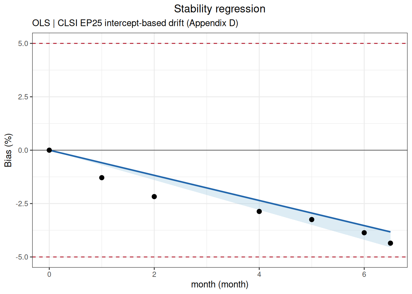
plot(ep25_c2_1_high_result)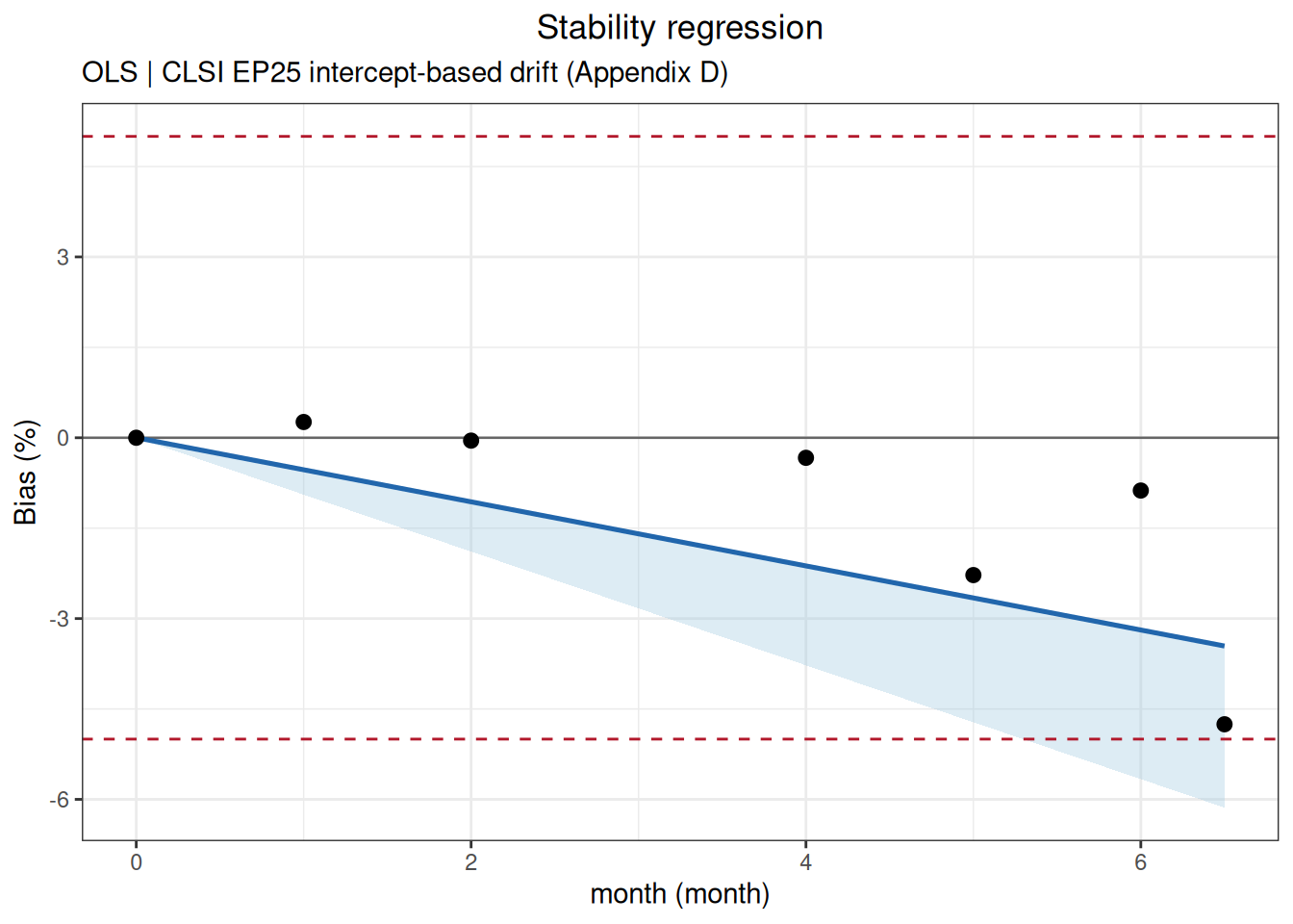
Compare the results with the standard:
| appendix | statistic | standard | ivdtools |
|---|---|---|---|
| EP25-A2 Appendix C2.1 / low_calibrator | change_6 | -3.53 | -3.532421 |
| EP25-A2 Appendix C2.1 / low_calibrator | change_6_upper_CL | -4.20 | -4.196768 |
| EP25-A2 Appendix C2.1 / low_calibrator | change_6.5 | -3.83 | -3.826789 |
| EP25-A2 Appendix C2.1 / low_calibrator | change_6.5_upper_CL | -4.55 | -4.546498 |
| EP25-A2 Appendix C2.1 / low_calibrator | ci_limit_time | 7.10 | 7.148359 |
| EP25-A2 Appendix C2.1 / high_calibrator | change_6 | -3.19 | -3.189971 |
| EP25-A2 Appendix C2.1 / high_calibrator | change_6_upper_CL | -5.66 | -5.664441 |
| EP25-A2 Appendix C2.1 / high_calibrator | change_6.5 | -3.46 | -3.455801 |
| EP25-A2 Appendix C2.1 / high_calibrator | change_6.5_upper_CL | -6.14 | -6.136478 |
| EP25-A2 Appendix C2.1 / high_calibrator | ci_limit_time | 5.30 | 5.296198 |
ep25_c2_2_data <- read_csv(
  "./data/004-稳定性研究/std-ep25-appendix-c2-2.csv",
  show_col_types = FALSE
)
head(ep25_c2_2_data, 6)
# A tibble: 6 × 3
level day result
<chr> <dbl> <dbl>
1 level_1 0 19.9
2 level_1 15 20.2
3 level_1 31 20.2
4 level_1 62 20.3
5 level_1 94 20.7
6 level_1 123 21.1ep25_c2_2_list <- split_by_factors(
ep25_c2_2_data,
variable = "level"
)
ep25_c2_2_list
Data split by factors
  Variable: level
  Groups: 3
  Missing/excluded: 0

  level_1  n = 9
  level_2  n = 9
  level_3  n = 9
Analyze the three calibrator levels sequentially with stability_regression():
ep25_c2_2_level_1_result <- stability_regression(
  data = ep25_c2_2_list$level_1,
  time = "day",
  value = "result",
  mode = "self",
  bias_type = "relative",
  direction = "increase",
  limit = 10,
  time_unit = "d",
  conf.level = 0.95
)

ep25_c2_2_level_2_result <- stability_regression(
  data = ep25_c2_2_list$level_2,
  time = "day",
  value = "result",
  mode = "self",
  bias_type = "relative",
  direction = "increase",
  limit = 10,
  time_unit = "d",
  conf.level = 0.95
)

ep25_c2_2_level_3_result <- stability_regression(
  data = ep25_c2_2_list$level_3,
  time = "day",
  value = "result",
  mode = "self",
  bias_type = "relative",
  direction = "increase",
  limit = 10,
  time_unit = "d",
  conf.level = 0.95
)

print(ep25_c2_2_level_1_result)
Stability Regression
  Mode:            self
  Test condition:  condition
  Fit:             OLS; intercept = 19.9291, slope = 0.0088
  Direction:       increase
  One-sided CI:    95.0%
  R-squared:       0.9789
  Note:            WLS unavailable; OLS used.

      Time      ObsBias   Estimate   CI_limit Status
  --------------------------------------------------
    0.0000       0.0000     0.0000     0.0000
   15.0000       1.5075     0.6616     0.7341
   31.0000       1.5075     1.3673     1.5171
   62.0000       2.0101     2.7345     3.0343
   94.0000       4.0201     4.1459     4.6003
  123.0000       6.0302     5.4249     6.0196
  154.0000       7.0352     6.7922     7.5367
  180.0000       8.5427     7.9389     8.8092
210.0000 9.0452 9.2620 10.2774 *print(ep25_c2_2_level_2_result)
Stability Regression
  Mode:            self
  Test condition:  condition
  Fit:             OLS; intercept = 100.9678, slope = 0.0292
  Direction:       increase
  One-sided CI:    95.0%
  R-squared:       0.9426
  Note:            WLS unavailable; OLS used.

      Time      ObsBias   Estimate   CI_limit Status
  --------------------------------------------------
    0.0000       0.0000     0.0000     0.0000
   15.0000       1.2859     0.4341     0.5129
   31.0000       0.3956     0.8970     1.0600
   62.0000       0.9891     1.7941     2.1201
   94.0000       2.3739     2.7201     3.2143
  123.0000       2.9674     3.5592     4.2060
  154.0000       4.1543     4.4563     5.2660
  180.0000       5.7369     5.2087     6.1551
210.0000 6.0336 6.0768 7.1809 print(ep25_c2_2_level_3_result)
Stability Regression
  Mode:            self
  Test condition:  condition
  Fit:             OLS; intercept = 502.3132, slope = 0.2573
  Direction:       increase
  One-sided CI:    95.0%
  R-squared:       0.9808
  Note:            WLS unavailable; OLS used.

      Time      ObsBias   Estimate   CI_limit Status
  --------------------------------------------------
    0.0000       0.0000     0.0000     0.0000
   15.0000       0.9014     0.7683     0.8491
   31.0000       2.8045     1.5878     1.7547
   62.0000       4.5873     3.1756     3.5094
   94.0000       5.6691     4.8147     5.3207
  123.0000       7.2516     6.3001     6.9622
  154.0000       8.2332     7.8879     8.7169
  180.0000       9.2147     9.2196    10.1886      *
210.0000 11.7388 10.7562 11.8867 *plot(ep25_c2_2_level_3_result)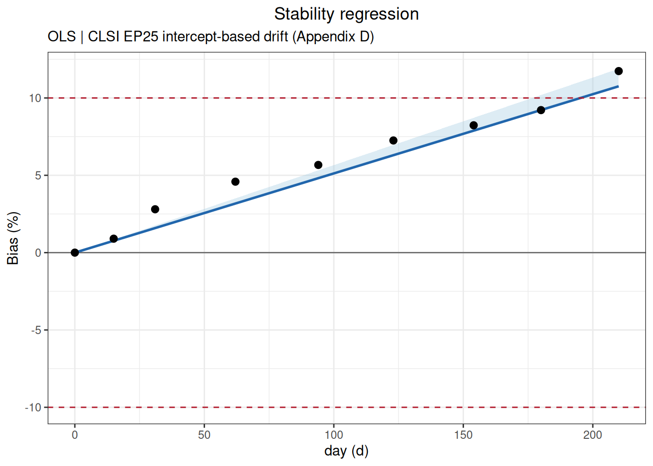
Compare the results with the standard:
| appendix | statistic | standard | ivdtools |
|---|---|---|---|
| EP25-A2 Appendix C2.2 / level_1 | change_180 | 7.97 | 7.938892 |
| EP25-A2 Appendix C2.2 / level_1 | change_180_upper_CL | 8.78 | 8.809166 |
| EP25-A2 Appendix C2.2 / level_1 | change_210 | 9.30 | 9.262041 |
| EP25-A2 Appendix C2.2 / level_1 | change_210_upper_CL | 10.24 | 10.277360 |
| EP25-A2 Appendix C2.2 / level_2 | change_180 | 5.19 | 5.208658 |
| EP25-A2 Appendix C2.2 / level_2 | change_180_upper_CL | 6.11 | 6.155086 |
| EP25-A2 Appendix C2.2 / level_2 | change_210 | 6.05 | 6.076767 |
| EP25-A2 Appendix C2.2 / level_2 | change_210_upper_CL | 7.13 | 7.180933 |
| EP25-A2 Appendix C2.2 / level_3 | change_180 | 9.19 | 9.219626 |
| EP25-A2 Appendix C2.2 / level_3 | change_180_upper_CL | 10.18 | 10.188639 |
| EP25-A2 Appendix C2.2 / level_3 | change_210 | 10.73 | 10.756231 |
| EP25-A2 Appendix C2.2 / level_3 | change_210_upper_CL | 11.87 | 11.886745 |
ep25_c3_1_data <- read_csv(
  "./data/004-稳定性研究/std-ep25-appendix-c3-1.csv",
  show_col_types = FALSE
)
head(ep25_c3_1_data, 6)
# A tibble: 6 × 4
control month condition result
<chr> <dbl> <chr> <dbl>
1 negative 0 reference 0.23
2 negative 1 reference 0.24
3 negative 2 reference 0.24
4 negative 3 reference 0.23
5 negative 4 reference 0.24
6 negative 5 reference 0.25ep25_c3_1_list <- split_by_factors(
ep25_c3_1_data,
variable = "control"
)
ep25_c3_1_list
Data split by factors
  Variable: control
  Groups: 2
  Missing/excluded: 0

  negative  n = 18
  positive  n = 18
Analyze the negative and positive controls separately with stability_regression():
ep25_c3_1_negative_result <- stability_regression(
  data = ep25_c3_1_list$negative,
  time = "month",
  value = "result",
  condition = "condition",
  mode = "compare",
  test_condition = "on_test",
  reference_condition = "reference",
  bias_type = "absolute",
  direction = "increase",
  limit = 0.10,
  time_unit = "month",
  conf.level = 0.95
)

ep25_c3_1_positive_result <- stability_regression(
  data = ep25_c3_1_list$positive,
  time = "month",
  value = "result",
  condition = "condition",
  mode = "compare",
  test_condition = "on_test",
  reference_condition = "reference",
  bias_type = "relative",
  direction = "decrease",
  limit = 5,
  time_unit = "month",
  conf.level = 0.95
)

print(ep25_c3_1_negative_result)
Stability Regression
  Mode:            compare
  Test condition:  on_test
  Reference:       reference
  Fit:             OLS; intercept = 0.0004, slope = 0.0103
  Direction:       increase
  One-sided CI:    95.0%
  R-squared:       0.8962
  Note:            WLS unavailable; OLS used.

      Time      ObsBias   Estimate   CI_limit Status
  --------------------------------------------------
    0.0000       0.0000     0.0004     0.0121
    1.0000       0.0200     0.0107     0.0204
    2.0000       0.0300     0.0210     0.0290
    3.0000       0.0200     0.0314     0.0381
    4.0000       0.0300     0.0417     0.0480
    5.0000       0.0400     0.0520     0.0588
    6.0000       0.0700     0.0623     0.0705
    7.0000       0.0800     0.0727     0.0826
7.5000 0.0800 0.0778 0.0888 print(ep25_c3_1_positive_result)
Stability Regression
  Mode:            compare
  Test condition:  on_test
  Reference:       reference
  Fit:             OLS; intercept = -0.0461, slope = -0.3655
  Direction:       decrease
  One-sided CI:    95.0%
  R-squared:       0.7765
  Note:            WLS unavailable; OLS used.

      Time      ObsBias   Estimate   CI_limit Status
  --------------------------------------------------
    0.0000      -0.1992    -0.0461    -0.7018
    1.0000      -0.5988    -0.4116    -0.9539
    2.0000      -0.8016    -0.7772    -1.2218
    3.0000      -1.3917    -1.1427    -1.5179
    4.0000      -1.3972    -1.5082    -1.8593
    5.0000      -0.8048    -1.8738    -2.2547
    6.0000      -1.8036    -2.2393    -2.6937
    7.0000      -2.7944    -2.6048    -3.1591
7.5000 -3.6000 -2.7876 -3.3979 plot(ep25_c3_1_negative_result)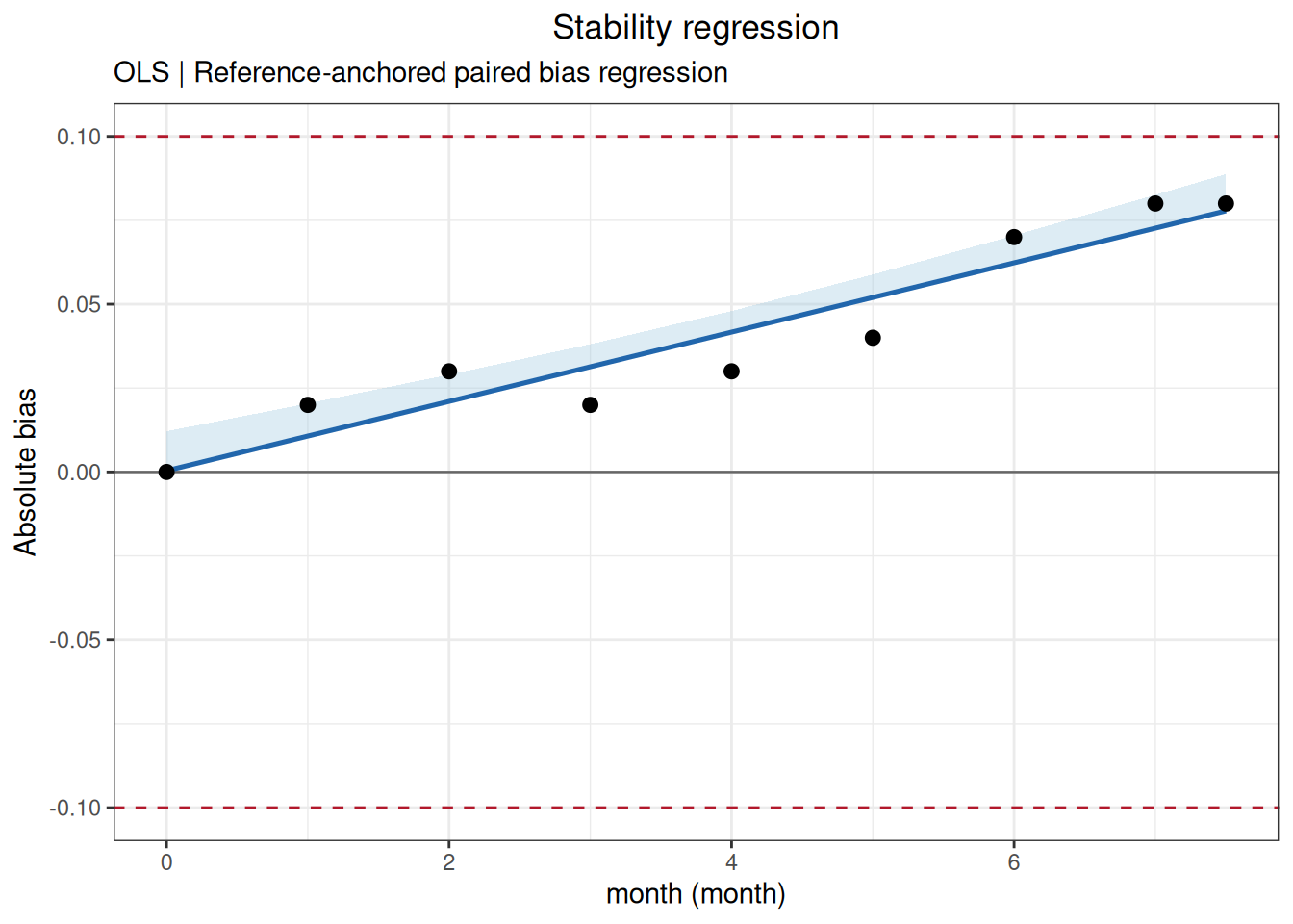
Compare the results with the standard:
| appendix | statistic | standard | ivdtools |
|---|---|---|---|
| EP25-A2 Appendix C3.1 / negative_control | change_7 | 0.07 | 0.072663 |
| EP25-A2 Appendix C3.1 / negative_control | change_7_upper_CL | 0.09 | 0.082595 |
| EP25-A2 Appendix C3.1 / negative_control | change_7.5 | 0.08 | 0.077826 |
| EP25-A2 Appendix C3.1 / negative_control | change_7.5_upper_CL | 0.10 | 0.088761 |
| EP25-A2 Appendix C3.1 / positive_control | change_7 | -2.56 | -2.604835 |
| EP25-A2 Appendix C3.1 / positive_control | change_7_upper_CL | -3.53 | -3.159133 |
| EP25-A2 Appendix C3.1 / positive_control | change_7.5 | -2.74 | -2.787602 |
| EP25-A2 Appendix C3.1 / positive_control | change_7.5_upper_CL | -3.79 | -3.397864 |
For the negative control, use absolute bias with a 0.10 IU/mL limit; for the positive control, use relative bias with a 5% limit.
ep25_c3_2_data <- read_csv(
  "./data/004-稳定性研究/std-ep25-appendix-c3-2.csv",
  show_col_types = FALSE
)
head(ep25_c3_2_data, 6)
# A tibble: 6 × 3
level day result
<chr> <dbl> <dbl>
1 level_1 0 1.21
2 level_1 40 1.17
3 level_1 80 1.22
4 level_1 120 1.18
5 level_1 162 1.15
6 level_1 203 1.14ep25_c3_2_list <- split_by_factors(
ep25_c3_2_data,
variable = "level"
)
ep25_c3_2_list
Data split by factors
  Variable: level
  Groups: 3
  Missing/excluded: 0

  level_1  n = 10
  level_2  n = 10
  level_3  n = 10
Analyze the three control levels sequentially with stability_regression():
ep25_c3_2_level_1_result <- stability_regression(
  data = ep25_c3_2_list$level_1,
  time = "day",
  value = "result",
  mode = "self",
  bias_type = "relative",
  direction = "decrease",
  limit = 10,
  time_unit = "d",
  conf.level = 0.95
)

ep25_c3_2_level_2_result <- stability_regression(
  data = ep25_c3_2_list$level_2,
  time = "day",
  value = "result",
  mode = "self",
  bias_type = "relative",
  direction = "decrease",
  limit = 10,
  time_unit = "d",
  conf.level = 0.95
)

ep25_c3_2_level_3_result <- stability_regression(
  data = ep25_c3_2_list$level_3,
  time = "day",
  value = "result",
  mode = "self",
  bias_type = "relative",
  direction = "decrease",
  limit = 10,
  time_unit = "d",
  conf.level = 0.95
)

print(ep25_c3_2_level_1_result)
Stability Regression
  Mode:            self
  Test condition:  condition
  Fit:             OLS; intercept = 1.2060, slope = -0.0003
  Direction:       decrease
  One-sided CI:    95.0%
  R-squared:       0.7575
  Note:            WLS unavailable; OLS used.

      Time      ObsBias   Estimate   CI_limit Status
  --------------------------------------------------
    0.0000       0.0000    -0.0000    -0.0000
   40.0000      -3.3058    -0.9917    -1.3431
   80.0000       0.8264    -1.9833    -2.6861
  120.0000      -2.4793    -2.9750    -4.0292
  162.0000      -4.9587    -4.0162    -5.4394
  203.0000      -5.7851    -5.0327    -6.8160
  255.0000      -8.2645    -6.3219    -8.5620
  305.0000     -10.7438    -7.5614   -10.2408      *
  364.0000      -6.6116    -9.0241   -12.2218      *
410.0000 -9.9174 -10.1645 -13.7663 *print(ep25_c3_2_level_2_result)
Stability Regression
  Mode:            self
  Test condition:  condition
  Fit:             OLS; intercept = 3.4233, slope = -0.0012
  Direction:       decrease
  One-sided CI:    95.0%
  R-squared:       0.9402
  Note:            WLS unavailable; OLS used.

      Time      ObsBias   Estimate   CI_limit Status
  --------------------------------------------------
    0.0000       0.0000    -0.0000    -0.0000
   40.0000       0.8798    -1.3939    -1.6098
   80.0000      -2.3460    -2.7879    -3.2195
  120.0000      -5.5718    -4.1818    -4.8293
  162.0000      -4.1056    -5.6454    -6.5195
  203.0000      -6.7449    -7.0742    -8.1695
  255.0000     -10.2639    -8.8863   -10.2622      *
  305.0000     -11.1437   -10.6287   -12.2744      *
  364.0000     -11.7302   -12.6847   -14.6488      *
410.0000 -12.9032 -14.2877 -16.5001 *print(ep25_c3_2_level_3_result)
Stability Regression
  Mode:            self
  Test condition:  condition
  Fit:             OLS; intercept = 7.5028, slope = -0.0016
  Direction:       decrease
  One-sided CI:    95.0%
  R-squared:       0.9912
  Note:            WLS unavailable; OLS used.

      Time      ObsBias   Estimate   CI_limit Status
  --------------------------------------------------
    0.0000       0.0000    -0.0000    -0.0000
   40.0000      -0.9321    -0.8327    -0.8822
   80.0000      -1.5979    -1.6653    -1.7645
  120.0000      -2.6631    -2.4980    -2.6467
  162.0000      -3.1957    -3.3723    -3.5731
  203.0000      -4.5273    -4.2258    -4.4774
  255.0000      -5.8589    -5.3083    -5.6243
  305.0000      -6.7909    -6.3491    -6.7271
  364.0000      -7.3236    -7.5773    -8.0285
410.0000 -8.3888 -8.5348 -9.0431 plot(ep25_c3_2_level_2_result)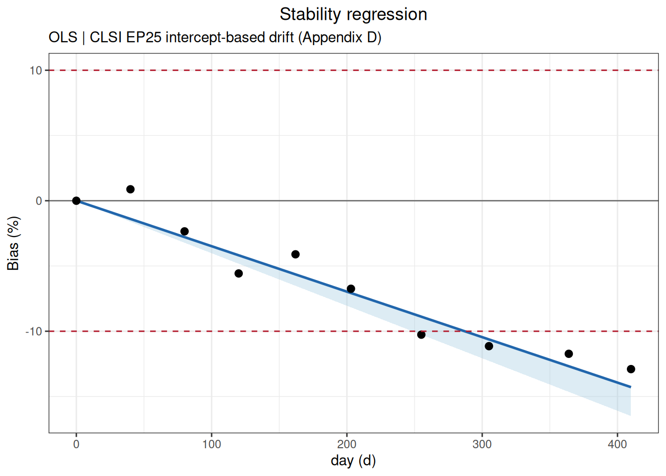
Compare the results with the standard:
| appendix | statistic | standard | ivdtools |
|---|---|---|---|
| EP25-A2 Appendix C3.2 / level_1 | change_364 | -9.00 | -9.024133 |
| EP25-A2 Appendix C3.2 / level_1 | change_364_upper_CL | -12.19 | -12.221806 |
| EP25-A2 Appendix C3.2 / level_1 | change_410 | -10.14 | -10.164545 |
| EP25-A2 Appendix C3.2 / level_1 | change_410_upper_CL | -13.73 | -13.766320 |
| EP25-A2 Appendix C3.2 / level_2 | change_364 | -12.68 | -12.684724 |
| EP25-A2 Appendix C3.2 / level_2 | change_364_upper_CL | -14.66 | -14.648829 |
| EP25-A2 Appendix C3.2 / level_2 | change_410 | -14.28 | -14.287738 |
| EP25-A2 Appendix C3.2 / level_2 | change_410_upper_CL | -16.52 | -16.500055 |
| EP25-A2 Appendix C3.2 / level_3 | change_364 | -7.58 | -7.577276 |
| EP25-A2 Appendix C3.2 / level_3 | change_364_upper_CL | -8.05 | -8.028464 |
| EP25-A2 Appendix C3.2 / level_3 | change_410 | -8.54 | -8.534844 |
| EP25-A2 Appendix C3.2 / level_3 | change_410_upper_CL | -9.07 | -9.043050 |
All three control levels use relative bias, decreasing direction, and a 10% allowable change. The comparison uses node estimates and one-sided confidence limits returned directly by the function.
ep25_c4_data <- read_csv(
  "./data/004-稳定性研究/std-ep25-appendix-c4.csv",
  show_col_types = FALSE
)
head(ep25_c4_data, 6)
# A tibble: 6 × 5
sample condition time replicate result
<chr> <chr> <dbl> <dbl> <dbl>
1 low_panel unstressed 0 1 7.24
2 low_panel unstressed 0 2 6.98
3 low_panel unstressed 0 3 6.94
4 low_panel unstressed 0 4 6.82
5 low_panel unstressed 0 5 7.09
6 low_panel unstressed 0 6 7.14ep25_c4_list <- split_by_factors(
ep25_c4_data,
variable = "sample"
)
ep25_c4_list
Data split by factors
  Variable: sample
  Groups: 3
  Missing/excluded: 0

  low_panel     n = 20
  low_control   n = 20
  high_control  n = 20
Evaluate the three samples separately with stability_bias():
ep25_c4_low_panel_result <- stability_bias(
  data = ep25_c4_list$low_panel,
  condition = "condition",
  time = "time",
  value = "result",
  reference_condition = "unstressed",
  limit = 5,
  bias_type = "relative",
  time_unit = "d"
)

ep25_c4_low_control_result <- stability_bias(
  data = ep25_c4_list$low_control,
  condition = "condition",
  time = "time",
  value = "result",
  reference_condition = "unstressed",
  limit = 5,
  bias_type = "relative",
  time_unit = "d"
)

ep25_c4_high_control_result <- stability_bias(
  data = ep25_c4_list$high_control,
  condition = "condition",
  time = "time",
  value = "result",
  reference_condition = "unstressed",
  limit = 5,
  bias_type = "relative",
  time_unit = "d"
)

print(ep25_c4_low_panel_result)
Stability Bias Analysis
  Conditions:      2 (unstressed, stressed)
  Reference:       unstressed
  Time unit:       d
  Node comparisons:0
  Acceptance:      +/- 5.0000 (relative); 2/2 nodes passed

  Within-condition bias (vs first node)
  Cond         Time      Value    Bias(%) Status
  ----------------------------------------------
  unstressed   0.0000     7.0710     0.0000 Pass
  stressed   0.0000     7.0700     0.0000 Pass

  Between-condition bias (reference: unstressed)
      Time Condition    TestVal  Bias(%)
  --------------------------------------
0.0000 stressed 7.0700 -0.0141print(ep25_c4_low_control_result)
Stability Bias Analysis
  Conditions:      2 (unstressed, stressed)
  Reference:       unstressed
  Time unit:       d
  Node comparisons:0
  Acceptance:      +/- 5.0000 (relative); 2/2 nodes passed

  Within-condition bias (vs first node)
  Cond         Time      Value    Bias(%) Status
  ----------------------------------------------
  unstressed   0.0000    25.1740     0.0000 Pass
  stressed   0.0000    25.1630     0.0000 Pass

  Between-condition bias (reference: unstressed)
      Time Condition    TestVal  Bias(%)
  --------------------------------------
0.0000 stressed 25.1630 -0.0437print(ep25_c4_high_control_result)
Stability Bias Analysis
  Conditions:      2 (unstressed, stressed)
  Reference:       unstressed
  Time unit:       d
  Node comparisons:0
  Acceptance:      +/- 5.0000 (relative); 2/2 nodes passed

  Within-condition bias (vs first node)
  Cond         Time      Value    Bias(%) Status
  ----------------------------------------------
  unstressed   0.0000    99.1610     0.0000 Pass
  stressed   0.0000    99.6930     0.0000 Pass

  Between-condition bias (reference: unstressed)
      Time Condition    TestVal  Bias(%)
  --------------------------------------
    0.0000 stressed    99.6930     0.5365
Compare the results with the standard:
| appendix | statistic | standard | ivdtools |
|---|---|---|---|
| EP25-A2 Appendix C4 / low_panel | relative_bias | 0.0 | -0.014142 |
| EP25-A2 Appendix C4 / low_control | relative_bias | 0.0 | -0.043696 |
| EP25-A2 Appendix C4 / high_control | relative_bias | 0.5 | 0.536501 |
The transport-condition example uses the reference-condition comparison returned by stability_bias(). The standard also reports confidence intervals for replicate measurements, but this function’s between_bias output does not include that item; therefore the comparison table lists only the relative bias returned directly by the function.
Read and inspect the standard data:
ep25_c5_data <- read_csv(
  "./data/004-稳定性研究/std-ep25-appendix-c5.csv",
  show_col_types = FALSE
)
head(ep25_c5_data, 6)
# A tibble: 6 × 2
Day Result
<dbl> <dbl>
1 0 12.1
2 31 12.0
3 61 15.0
4 96 11.9
5 120 11.8
6 150 11.8ep25_c5_without_day_61 <- ep25_c5_data[ep25_c5_data$Day != 61, ]
head(ep25_c5_without_day_61, 6)# A tibble: 6 × 2
Day Result
<dbl> <dbl>
1 0 12.1
2 31 12.0
3 96 11.9
4 120 11.8
5 150 11.8
6 186 11.8Use stability_regression() to evaluate the results with and without the outlier:
ep25_c5_with_result <- stability_regression(
  data = ep25_c5_data,
  time = "Day",
  value = "Result",
  mode = "self",
  bias_type = "relative",
  direction = "decrease",
  limit = 10,
  time_unit = "d",
  conf.level = 0.95
)

ep25_c5_without_result <- stability_regression(
  data = ep25_c5_without_day_61,
  time = "Day",
  value = "Result",
  mode = "self",
  bias_type = "relative",
  direction = "decrease",
  limit = 10,
  time_unit = "d",
  conf.level = 0.95
)

print(ep25_c5_with_result)
Stability Regression
  Mode:            self
  Test condition:  condition
  Fit:             OLS; intercept = 12.6703, slope = -0.0035
  Direction:       decrease
  One-sided CI:    95.0%
  R-squared:       0.2118
  Cook distance:   row(s) 3 > 1; not removed
  Note:            WLS unavailable; OLS used.

      Time      ObsBias   Estimate   CI_limit Status
  --------------------------------------------------
    0.0000       0.0000    -0.0000    -0.0000
   31.0000      -0.7432    -0.8643    -1.7218
   61.0000      23.7820    -1.7008    -3.3880
   96.0000      -2.0644    -2.6766    -5.3320
  120.0000      -2.2296    -3.3457    -6.6650
  150.0000      -2.8076    -4.1822    -8.3313
  186.0000      -2.3947    -5.1859   -10.3308      *
  211.0000      -2.6424    -5.8829   -11.7193      *
  233.0000      -4.0462    -6.4963   -12.9412      *
  270.0000      -3.2205    -7.5279   -14.9963      *
  301.0000      -3.7985    -8.3922   -16.7181      *
  333.0000      -4.1288    -9.2844   -18.4954      *
370.0000 -4.4591 -10.3160 -20.5504 *print(ep25_c5_without_result)
Stability Regression
  Mode:            self
  Test condition:  condition
  Fit:             OLS; intercept = 12.0369, slope = -0.0013
  Direction:       decrease
  One-sided CI:    95.0%
  R-squared:       0.8969
  Note:            WLS unavailable; OLS used.

      Time      ObsBias   Estimate   CI_limit Status
  --------------------------------------------------
    0.0000       0.0000    -0.0000    -0.0000
   31.0000      -0.7432    -0.3428    -0.4080
   96.0000      -2.0644    -1.0615    -1.2634
  120.0000      -2.2296    -1.3269    -1.5793
  150.0000      -2.8076    -1.6586    -1.9741
  186.0000      -2.3947    -2.0567    -2.4479
  211.0000      -2.6424    -2.3331    -2.7769
  233.0000      -4.0462    -2.5764    -3.0665
  270.0000      -3.2205    -2.9855    -3.5534
  301.0000      -3.7985    -3.3283    -3.9614
  333.0000      -4.1288    -3.6821    -4.3826
370.0000 -4.4591 -4.0912 -4.8695 plot(ep25_c5_with_result)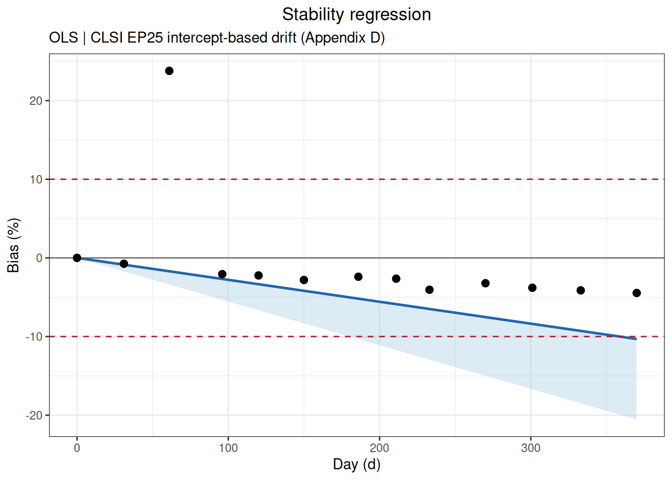
Cook’s distance:
stability_regression() calculates Cook’s distance for each time point in the returned object and records observations with Cook’s distance greater than 1 in diagnostics$influential:
ep25_c5_cook_distance <- data.frame(
  Day = ep25_c5_data$Day,
  Cook_distance = unname(ep25_c5_with_result$diagnostics$cook_distance)
)
ep25_c5_cook_distance
Day Cook_distance
1 0 1.172637e-01
2 31 7.185586e-02
3 61 1.078556e+00
4 96 2.477807e-02
5 120 1.448582e-02
6 150 9.639484e-03
7 186 2.404885e-03
8 211 1.263118e-03
9 233 4.142662e-03
10 270 1.404264e-06
11 301 3.051755e-04
12 333 3.335777e-03
13 370 1.752518e-02ep25_c5_influential <- ep25_c5_cook_distance[
ep25_c5_cook_distance$Cook_distance > 1,
]
ep25_c5_influential Day Cook_distance
3 61 1.078556Compare the results with the standard:
| appendix | statistic | standard | ivdtools |
|---|---|---|---|
| EP25-A2 Appendix C5 / with_outlier | cook_distance_day_61 | 1.08 | 1.078556 |
| EP25-A2 Appendix C5 / with_outlier | change_333 | -9.28 | -9.284424 |
| EP25-A2 Appendix C5 / with_outlier | change_333_upper_CL | -18.50 | -18.495388 |
| EP25-A2 Appendix C5 / with_outlier | change_370 | -10.32 | -10.316027 |
| EP25-A2 Appendix C5 / with_outlier | change_370_upper_CL | -20.55 | -20.550431 |
| EP25-A2 Appendix C5 / without_day_61 | change_333 | -3.68 | -3.682110 |
| EP25-A2 Appendix C5 / without_day_61 | change_333_upper_CL | -4.38 | -4.382553 |
| EP25-A2 Appendix C5 / without_day_61 | change_370 | -4.09 | -4.091233 |
| EP25-A2 Appendix C5 / without_day_61 | change_370_upper_CL | -4.87 | -4.869504 |